Week 2 — Tests as decision rules and the Neyman-Pearson lemma

Where this week starts

Last week put every procedure inside one frame: an estimand, an action space, a loss function, a rule \(\delta\) from data to action, and a risk function \(R(\theta, \delta)\) reporting what the rule costs at each parameter value. It ended uncomfortably. Risk is a function of \(\theta\), most pairs of procedures are not comparable under it, and nothing in the frame said how to choose. This week takes the smallest interesting special case and shows how a choice becomes possible there.

The special case is testing. The action space has two elements, reject and do not reject; the parameter space splits into a null set \(\Theta_0\) and an alternative set \(\Theta_1\); and the loss charges only for the two ways of being wrong. What makes testing tractable is a deliberate asymmetry: rather than making both error probabilities small at once, you cap one and maximize over the other. That is a modelling decision, not a mathematical necessity, and much of what students find strange about testing follows from it.

The reward is the Week 1 ordering problem solved outright in one case. Among all tests whose probability of rejecting a simple null does not exceed \(\alpha\), the Neyman-Pearson lemma names a single best one against a simple alternative and shows there is nothing left to argue about. That is rare here, and it is worth seeing how narrow the conditions are that buy it: one null point, one alternative point, and a level fixed in advance.

By the end of this page, three phrases you have used loosely should have separated. Level is a promise you make; size is what your test actually does; power is a whole function, not a number.

Why this matters beyond the theorem

Consider a clinical laboratory validating a new assay against a reference method. The team runs a level 0.05 test, rejects, and writes that “at most five percent of the results we report this way are false alarms”. That is a different probability from the one the level controls: the level bounds the chance of rejecting given that the null is true, while the sentence is about how often a rejection is wrong, which also depends on how often the nulls tested are true. Suppose the laboratory runs a thousand such comparisons, nine hundred involving no real difference, and its test has power 0.80 where a difference exists. Then it rejects about \(900 \times 0.05 = 45\) times when nothing is there and about \(100 \times 0.80 = 80\) times when something is, so roughly \(45 / 125\), or thirty-six percent, of its rejections are false alarms — seven times the figure it reported.

Nothing there is subtle and no simulation is needed; it follows from taking the definition of size literally and noticing which conditioning it fixes.

What you will be able to do

• Write a testing problem as a null set \(\Theta_0\), an alternative set \(\Theta_1\), and a test function \(\varphi\), and identify the loss that makes it a decision problem in last week’s sense.
• Compute the power function \(\beta(\theta) = E_\theta \varphi(X)\) of a stated test, and read the size off it as a supremum rather than as a value at one convenient point.
• Distinguish size from level, and exhibit a test whose rejection probability at one null value is 0.05 while its size is far larger.
• Derive the most powerful test of a simple null against a simple alternative from the likelihood ratio, and state the conditions the Neyman-Pearson lemma actually requires.
• Prove the sufficiency direction of the lemma from the pointwise inequality it turns on, and say which step fails if the threshold is allowed to be negative.
• Construct a randomized test of exact size in a discrete model, compute the randomization probability, and audit a written interpretation of a p-value against the definitions.

Terms and notation worth fixing

The rest of the course reuses these symbols without reintroducing them. Every one is a property of a procedure and a model, never of a data set.

Symbol or term	Meaning as used in this course
\(\Theta_0\), \(\Theta_1\)	the null and alternative subsets of \(\Theta\); they are disjoint and their union is the parameter space under discussion
\(\varphi(x)\)	the test function: the probability of rejecting when the data are \(x\), so \(\varphi\) maps the sample space into the interval from zero to one
non-randomized test	a test with \(\varphi(x)\) equal to zero or one everywhere; its rejection region is \(\{x : \varphi(x) = 1\}\)
\(\beta(\theta)\)	the power function \(E_\theta \varphi(X)\), defined at every \(\theta \in \Theta\), null values included
size	\(\sup_{\theta \in \Theta_0} \beta(\theta)\): the worst rejection probability the null set allows
level \(\alpha\)	a number chosen in advance that the size does not exceed; a level is a promise, and many tests keep it
type I, type II error	rejecting when \(\theta \in \Theta_0\), and failing to reject when \(\theta \in \Theta_1\); their probabilities are \(\beta(\theta)\) and \(1 - \beta(\theta)\)
\(\Lambda(x)\), \(k\), \(\gamma\)	the likelihood ratio \(f_1(x) / f_0(x)\), the threshold it is compared with, and the probability of rejecting when the ratio lands exactly on the threshold

A test is a decision rule with two error rates

Fix a model \(\{P_\theta : \theta \in \Theta\}\) and a partition of \(\Theta\) into \(\Theta_0\) and \(\Theta_1\). A test is a procedure in exactly last week’s sense, with action space \(\{\text{reject}, \text{do not reject}\}\) and the zero-one loss on it: no loss for the right action, one unit for either mistake. Under that loss the risk is \(\beta(\theta)\) on \(\Theta_0\) and \(1 - \beta(\theta)\) on \(\Theta_1\), so the whole risk function is carried by one object, the power function.

The test function and the two ways to be wrong

Allowing \(\varphi\) to take values strictly between zero and one looks like an eccentricity, and for the continuous models on this page it is: no such test is ever needed. Its purpose is to make the family of tests convex, so that this week’s optimization has a solution in discrete models too. Read \(\varphi(x)\) as an instruction: observe \(x\), then reject with probability \(\varphi(x)\), using a randomization independent of the data. When \(\varphi\) takes only the values zero and one it is the indicator of a rejection region and no auxiliary device is used.

The two errors are not symmetric in the theory, and it is worth being blunt about why. No principle of statistics makes a false rejection worse than a false retention; that ranking comes from the scientific setting, and a decision-theoretic treatment would put the two losses in a ratio and minimize expected loss, as last week’s batch-acceptance example did. Testing caps the first error instead, because the null is often sharp while the alternative is a vague direction, and because a cap needs no ratio of costs you may not know.

Size, level, and the supremum you must not drop

The power function \(\beta(\theta) = E_\theta \varphi(X)\) is defined at every \(\theta\), and on \(\Theta_0\) it reports the probability of a type I error at that particular \(\theta\). The size is the supremum of those numbers over the whole null set, and a test has level \(\alpha\) when its size is at most \(\alpha\). Two consequences follow at once and are constantly forgotten. First, level is not a property a test has uniquely: a test of size 0.01 has level 0.05, level 0.10, and level 0.5, so calling it a level 0.05 test says only that it keeps a promise. Second, when \(\Theta_0\) has more than one point, the rejection probability at one convenient null value proves nothing about the size, because the supremum may be attained elsewhere or not attained at all.

For a simple null, \(\Theta_0 = \{\theta_0\}\), the supremum is over one point and the size is just \(\beta(\theta_0)\). That is why this week’s theorem is stated for a simple null: the complication is postponed, not solved. Week 3 returns to it for one-sided composite nulls, where a monotone power function puts the supremum at the boundary, and Week 6 for nulls carrying nuisance parameters, where it is genuinely hard.

The power function is the object of study

Power is a function, and almost every confusion this week dissolves once that is taken literally. One test has a different power at each alternative, so “the power of the test” is an incomplete phrase until an alternative and a sample size are named.

The power function of a one-sided level 0.05 test of a normal mean, drawn at two sample sizes.

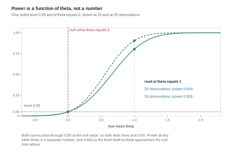
Three features of that picture are worth naming. The curve passes through the level exactly at the null value, which is what having size 0.05 means here. It falls continuously to the level as the alternative approaches the null, so at a fixed sample size no test has high power against alternatives arbitrarily close to \(\theta_0\); a claim of high power must name an alternative far enough away to matter. And more observations lift the whole curve while leaving the null value pinned at 0.05, which is the only way to improve both error rates at once.

The Neyman-Pearson lemma and what it costs

Now restrict to the simplest problem: \(\Theta_0 = \{\theta_0\}\) and \(\Theta_1 = \{\theta_1\}\), both simple. Write \(f_0\) and \(f_1\) for the two densities with respect to a common \(\sigma\)-finite measure \(\mu\) dominating both — Lebesgue measure for continuous models, counting measure for discrete ones — and let \(\Lambda(x) = f_1(x) / f_0(x)\) be the likelihood ratio, with \(\Lambda(x) = \infty\) where \(f_0(x) = 0\) and \(f_1(x) > 0\). Fix \(\alpha \in (0, 1)\).

Lemma (Neyman and Pearson). Existence. There exist a constant \(k \ge 0\) and a number \(\gamma \in [0, 1]\) such that the test

\[ \varphi^*(x) = \begin{cases} 1, & \Lambda(x) > k, \\ \gamma, & \Lambda(x) = k, \\ 0, & \Lambda(x) < k, \end{cases} \]

satisfies \(E_{\theta_0} \varphi^*(X) = \alpha\) exactly. Sufficiency. Any test of that form with size \(\alpha\) is most powerful at level \(\alpha\): every test \(\varphi\) with \(E_{\theta_0} \varphi(X) \le \alpha\) has \(E_{\theta_1} \varphi^*(X) \ge E_{\theta_1} \varphi(X)\). Necessity. If \(\varphi\) is most powerful at level \(\alpha\), it agrees with \(\varphi^*\) almost everywhere with respect to \(\mu\) on the set where \(\Lambda(x) \ne k\).

The cases are usually written as comparisons of \(f_1(x)\) with \(k f_0(x)\) rather than of \(\Lambda(x)\) with \(k\). The two agree: where \(f_0(x) > 0\) they are one inequality divided by \(f_0(x)\), and where \(f_0(x) = 0\) the convention \(\Lambda = \infty\) rejects, exactly as \(f_1(x) > k f_0(x) = 0\) does. The proof below uses the second form because it integrates.

Notice what is not assumed: nothing about normality, exponential families, sample size, independence, or continuity, nothing asymptotic, no regularity conditions on derivatives of the likelihood. The price is the narrowness of the problem, one null point and one alternative point; Weeks 3 through 6 keep some of the conclusion while widening the hypothesis.

The binomial likelihood ratio against the number of successes, with the Neyman-Pearson threshold marked.

Existence is a construction, not an abstraction, and worth doing once. Let \(G(t) = P_{\theta_0}(\Lambda(X) > t)\), a non-increasing right-continuous function falling from at most one to zero, and take \(k = \inf\{t \ge 0 : G(t) \le \alpha\}\). Then \(G(k) \le \alpha\) and the left limit of \(G\) at \(k\) is at least \(\alpha\); since that left limit equals \(G(k) + P_{\theta_0}(\Lambda(X) = k)\), the shortfall \(\alpha - G(k)\) never exceeds \(P_{\theta_0}(\Lambda(X) = k)\). So put

\[ \gamma = \frac{\alpha - G(k)}{P_{\theta_0}(\Lambda(X) = k)} \]

when that denominator is positive, and let \(\gamma\) be anything otherwise. Then \(E_{\theta_0} \varphi^* = G(k) + \gamma P_{\theta_0}(\Lambda(X) = k) = \alpha\). Whenever the ratio has a continuous null distribution — as it does in every continuous model on this page — that denominator is zero at every \(k\), \(G\) is continuous, and the shortfall is zero: randomization is available but never called on.

Proving that the ratio test cannot be beaten

The sufficiency proof is one inequality and one integration, and every later optimality argument in this course is a variation on it. Let \(\varphi^*\) be as above with \(E_{\theta_0}\varphi^* = \alpha\), and \(\varphi\) any test with \(E_{\theta_0}\varphi \le \alpha\). The claim is the pointwise inequality

\[ \big(\varphi^*(x) - \varphi(x)\big)\big(f_1(x) - k f_0(x)\big) \ge 0 \qquad \text{for every } x . \]

Check the three cases. Where \(f_1(x) > k f_0(x)\) the second factor is positive and \(\varphi^*(x) = 1 \ge \varphi(x)\), so the first factor is non-negative. Where \(f_1(x) < k f_0(x)\) the second factor is negative and \(\varphi^*(x) = 0 \le \varphi(x)\), so the first factor is non-positive; the product is again non-negative. Where \(f_1(x) = k f_0(x)\) the second factor vanishes and the product is zero regardless of \(\gamma\) — which is exactly why the lemma may leave \(\gamma\) free without harming optimality. Integrating a non-negative function against \(\mu\),

\[ 0 \le \int \big(\varphi^* - \varphi\big)\big(f_1 - k f_0\big) \, d\mu = \big(E_{\theta_1}\varphi^* - E_{\theta_1}\varphi\big) - k \big(E_{\theta_0}\varphi^* - E_{\theta_0}\varphi\big) . \]

The second bracket is \(\alpha - E_{\theta_0}\varphi \ge 0\), and \(k \ge 0\), so \(E_{\theta_1}\varphi^* - E_{\theta_1}\varphi \ge k(\alpha - E_{\theta_0}\varphi) \ge 0\). That is the claim. Two conditions did real work: \(k \ge 0\), without which the last inequality fails, and \(E_{\theta_0}\varphi \le \alpha\), the level restriction. Drop the level restriction and the test that always rejects has power one, so the theorem would be empty.

Necessity, ties, and the coin the lemma needs

Necessity comes free from the same display. Suppose \(\varphi\) is also most powerful at level \(\alpha\). Then \(E_{\theta_1}\varphi = E_{\theta_1}\varphi^*\), so the integral above equals \(-k(\alpha - E_{\theta_0}\varphi)\), which is at most zero; but its integrand is non-negative pointwise, so it is at least zero. Hence the integral is zero and the integrand vanishes \(\mu\)-almost everywhere. Wherever \(f_1(x) \ne k f_0(x)\) the second factor is non-zero, so \(\varphi = \varphi^*\) there. The lemma pins the test down everywhere except on the tie set, where any \(\gamma\) giving the right size will do.

That tie set is the whole story of randomization. In a discrete model the ratio takes countably many values, each with positive null probability, so \(G\) jumps and there is generally no \(k\) with \(G(k) = \alpha\) exactly. Refusing to randomize means settling for a size strictly below \(\alpha\) — a conservative test, and by the lemma a less powerful one. Randomizing means two analysts with identical data can reach different decisions, which is why no laboratory reports one. Randomized tests make the optimality statement exact; in practice the discreteness reappears as conservatism, which Week 4 meets again in the coverage of exact intervals.

Worked example — the most powerful test for a normal mean

Let \(X_1, \dots, X_{25}\) be independent \(N(\theta, \sigma^2)\) with \(\sigma = 2\) known, so \(n = 25\) and the standard error of the sample mean is \(\sigma / \sqrt{n} = 0.4\). Test \(H_0 : \theta = 0\) against \(H_1 : \theta = 1\). Both hypotheses are simple, so the lemma applies with no further conditions.

Step 1: form the ratio. Writing \(\bar{x}\) for the sample mean and cancelling the factors free of \(\theta\),

\[ \Lambda(x) = \frac{f_1(x)}{f_0(x)} = \exp\!\left\{ \frac{n}{\sigma^2}\left( (\theta_1 - \theta_0)\bar{x} - \frac{\theta_1^2 - \theta_0^2}{2} \right) \right\} = \exp\!\left\{ 6.25\, \bar{x} - 3.125 \right\} , \]

using \(n / \sigma^2 = 25/4 = 6.25\), \(\theta_1 - \theta_0 = 1\), and \((\theta_1^2 - \theta_0^2)/2 = 0.5\), so that the constant is \(6.25 \times 0.5 = 3.125\).

Step 2: reduce it. The exponential is strictly increasing, so \(\Lambda(x) > k\) if and only if \(\bar{x} > (\log k + 3.125) / 6.25\). The Neyman-Pearson region is therefore an upper tail of \(\bar{X}\), and the ratio never needs computing again: it depends on the data only through the sufficient statistic \(\bar{x}\).

Step 3: set the cutoff for exact size 0.05. Under \(H_0\), \(\bar{X} \sim N(0, 0.4^2)\). With \(z_{0.95} = 1.645\) to three decimals, the cutoff is \(c = 1.645 \times 0.4 = 0.658\). Since \(\bar{X}\) is continuous, \(P_{\theta_0}(\Lambda = k) = 0\) and \(\gamma\) is irrelevant; the size is exactly 0.05 with no randomization. On the ratio scale the threshold is \(k = \exp(6.25 \times 0.658 - 3.125) = \exp(0.9875) = 2.68\).

Step 4: compute the power at the alternative. Under \(H_1\), \(\bar{X} \sim N(1, 0.4^2)\), so

\[ \beta(1) = P_{\theta_1}(\bar{X} \ge 0.658) = 1 - \Phi\!\left( \frac{0.658 - 1}{0.4} \right) = 1 - \Phi(-0.855) = \Phi(0.855) = 0.804 . \]

The type II error probability is \(1 - 0.804 = 0.196\). The general power function is \(\beta(\theta) = \Phi\big((\theta - 0.658)/0.4\big)\), which returns \(\Phi(-1.645) = 0.05\) at the null, as it must.

Null and alternative densities of the sample mean with one cutoff and both error probabilities shaded.

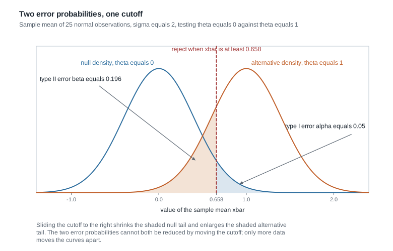
Step 5: say what this licenses. Among all tests of \(\theta = 0\) against \(\theta = 1\) whose null rejection probability is at most 0.05, including randomized ones, none has power above 0.804 at \(\theta = 1\). What it does not license is broader: 0.804 describes the procedure at one parameter value, not the data set you will collect, and the same test is nearly worthless against \(\theta = -0.5\), where \(\beta(-0.5) = \Phi(-2.895) = 0.002\). For power 0.90 at \(\theta = 1\), change the design rather than the arithmetic: solving \(\sqrt{n}/2 - 1.645 \ge 1.282\) gives \(\sqrt{n} \ge 5.854\), so \(n = 35\), at which the power is 0.905.

The same reasoning, transferred

Now let \(X_1, \dots, X_{10}\) be independent exponential lifetimes with density \(\theta e^{-\theta x}\) for \(x > 0\), and test \(H_0 : \theta = 1\) against \(H_1 : \theta = 1/2\) — a doubling of the mean lifetime. With \(S = \sum_i X_i\),

\[ \Lambda(x) = \frac{(1/2)^{10} e^{-S/2}}{1^{10} e^{-S}} = 2^{-10} \, e^{S/2} , \]

which is strictly increasing in \(S\), so the test again rejects on an upper tail of a one-dimensional sufficient statistic. Under \(H_0\), \(S\) has the gamma distribution with shape ten and rate one, and \(2S \sim \chi^2_{20}\). The 0.95 quantile of that chi-square is 31.41, so the exact level 0.05 cutoff is \(c = 15.71\); \(S\) is continuous, so again no randomization arises. Under \(H_1\) the scaling \(2\theta_1 S = S\) is itself \(\chi^2_{20}\), so the power is \(P(\chi^2_{20} \ge 15.71) = 0.734\), which pchisq(15.71, 20, lower.tail = FALSE) returns.

What stayed the same: the lemma, and the monotone reduction of the ratio to a sufficient statistic that makes continuity enough to avoid randomizing. What changed: the alternative has a smaller parameter than the null, yet the rejection region is still an upper tail — of \(S\), because long lifetimes are evidence for a low failure rate. The lemma orders the sample space by the ratio, never by the parameter, so read the direction off the ratio. The reference law also turned from symmetric to right-skewed, so the cutoff is no longer a tidy multiple of a standard error.

Second worked example — a binomial size you cannot hit

Let \(X \sim \text{Binomial}(10, \theta)\) and test \(H_0 : \theta = 0.5\) against \(H_1 : \theta = 0.7\). The binomial coefficients cancel in the ratio, leaving

\[ \Lambda(x) = \frac{\binom{10}{x} (0.7)^x (0.3)^{10-x}}{\binom{10}{x} (0.5)^{10}} = (1.4)^x (0.6)^{10-x} , \]

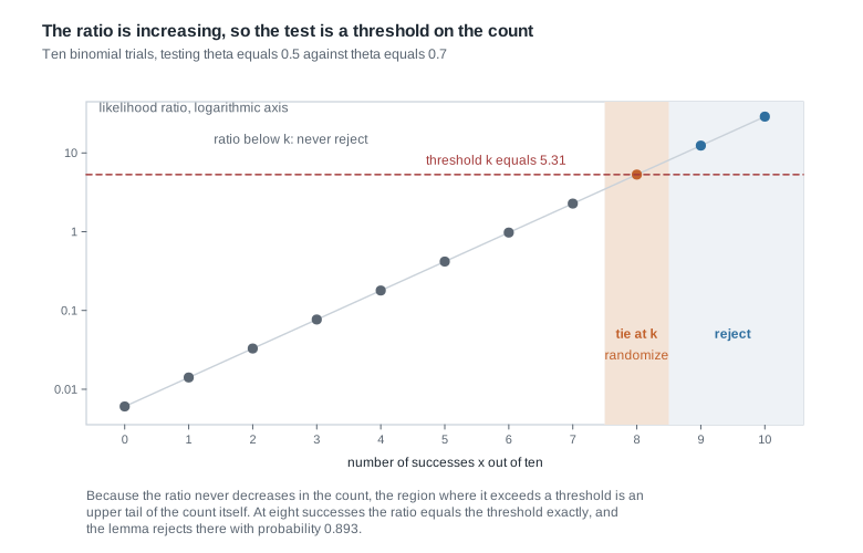
which increases in \(x\) because \(1.4 / 0.6 > 1\). So the region is again an upper tail, now of the count.

The obstruction. Under \(H_0\) every event has probability equal to a whole number of \(1024\)ths, since \(2^{10} = 1024\). But \(0.05 \times 1024 = 51.2\) is not a whole number, so no non-randomized test in this model has size exactly 0.05 — not merely no upper-tail test. The upper tails give \(P(X \ge 10) = 1/1024 = 0.0010\), \(P(X \ge 9) = 11/1024 = 0.0107\), and \(P(X \ge 8) = 56/1024 = 0.0547\). The wanted size falls in the gap.

Size of the non-randomized binomial test as a step function of the cutoff, with 0.05 in the gap.

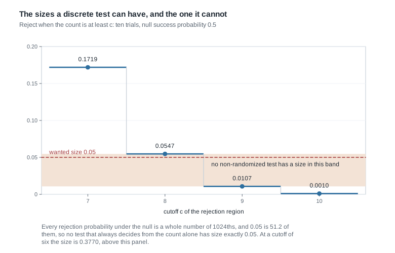
The randomized test. Take \(k = \Lambda(8) = (1.4)^8 (0.6)^2 = 5.31\). Then \(P_{\theta_0}(\Lambda > k) = P(X \ge 9) = 11/1024\) and \(P_{\theta_0}(\Lambda = k) = P(X = 8) = 45/1024\), so the existence construction gives

\[ \gamma = \frac{0.05 - 11/1024}{45/1024} = \frac{51.2 - 11}{45} = \frac{40.2}{45} = 0.893 . \]

The test rejects if \(X \ge 9\); if \(X = 8\) it rejects with probability 0.893, using a device independent of the data; otherwise it does not reject. Its size is \(11/1024 + 0.893 \times 45/1024 = 0.0500\).

What it buys. Under \(\theta = 0.7\) the relevant probabilities are \(P(X \ge 9) = 0.1493\) and \(P(X = 8) = 0.2335\), so the power is \(0.1493 + 0.893 \times 0.2335 = 0.358\). Compare the two non-randomized neighbours. The conservative test rejecting \(X \ge 9\) has size 0.0107 and power 0.149: it surrenders more than half the attainable power while using a fifth of the size it was allowed. The test rejecting \(X \ge 8\) has power 0.383, but its size is 0.0547, so it is not a level 0.05 test and the lemma says nothing in its defence. That is the honest picture of discreteness, and the cost shrinks only as the sample grows.

Auditing a stated error-rate claim

The definitions above are enough to audit most written conclusions, and doing that deliberately is what makes them stick. Here is a specimen of the kind produced fluently by hurried authors and text generators alike, invented rather than quoted.

Note

A claim to audit. “The comparison was significant at the 0.05 level, with a p-value of 0.032, so there is only about a three percent chance that the null hypothesis is true. At most five percent of the findings we report this way are false alarms. The study had power 0.80, so if the effect were real we would have detected it four times in five; we did detect it, so the effect is real with probability 0.80.”

Take the sentences in order. The p-value is \(p(x) = \sup_{\theta \in \Theta_0} P_\theta\big(T(X) \ge T(x)\big)\): a probability computed over data sets with \(\theta\) held fixed inside \(\Theta_0\), not a probability spread over \(\theta\), and converting it into one requires a prior, which is Week 14’s business. The second sentence reverses a conditioning, as the laboratory arithmetic above showed. The third treats power at one alternative as the probability that a rejection is correct — the same reversal applied to \(\beta\) — and as though it held at every alternative.

Power against size as the cutoff of the most powerful normal test slides.

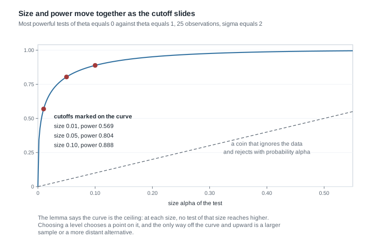
Only the first clause survives, and even that is a statement about the procedure. Sliding the cutoff moves you along the curve above and nowhere else, so tightening the level to 0.01 in this design drops the power from 0.804 to 0.569 and raises the type II error from 0.196 to 0.431. Reporting a level is reporting a choice about which error you were more willing to make. Computing that curve before collecting data is the calibration habit this course is building:

sigma <- 2; n <- 25; drift <- sqrt(n) * 1 / sigma   # 2.5 standard errors apart
alpha <- c(0.01, 0.05, 0.10)
pnorm(drift - qnorm(1 - alpha))                     # 0.569 0.804 0.888

The misreading to avoid

The misreading that survives longest sounds like this: “my test has level 0.05, so there is a five percent chance that the conclusion I just reached is a type I error.” The sentence is wrong twice over.

It is wrong first because the probability is attached to the wrong object. Once the data are in hand and the decision is made, either \(\theta \in \Theta_0\) or it is not, and either the decision is an error or it is not; the sampling randomness has been spent. The number 0.05 is the long-run frequency of rejection in repeated samples from a fixed \(\theta\) in \(\Theta_0\). If your null is in fact false, your probability of having committed a type I error is zero, not 0.05, and you do not know which case you are in. That is not a defect of testing; it is what a frequentist guarantee is.

It is wrong a second time because it treats a level as though it were the size. Take the same normal model, \(n = 25\) and \(\sigma = 2\), but test \(H_0 : \theta \le 0\) against \(H_1 : \theta > 0\) with the two-sided region rejecting when \(|\bar{X}| \ge 0.784\). At \(\theta = 0\) its rejection probability is \(2\big(1 - \Phi(1.96)\big) = 0.05\) exactly, so a reader who checks only the boundary point certifies it as a level 0.05 test. But at \(\theta = -1\), which lies in \(\Theta_0\), the rejection probability is at least \(\Phi\big((-0.784 + 1)/0.4\big) = \Phi(0.54) = 0.705\) from the lower tail alone, and as \(\theta\) runs to \(-\infty\) it tends to one. The size is one. A test can hit 0.05 on the nose at the boundary null value and still be worthless, and only the supremum detects it.

A third misreading shapes bad habits: “the Neyman-Pearson test is the best test.” It is most powerful against the one alternative it was built for, at the one level it was built at. In the normal example the cutoff 0.658 happened not to depend on \(\theta_1\), a structural accident that seeds next week’s theory; in general the optimal test moves with the alternative, as the power 0.002 against \(\theta = -0.5\) shows.

Practice on your own

These are for self-checking, not submission, and are best worked with the definitions in front of you.

1. A discrete derivation. Let \(X_1, \dots, X_{10}\) be independent Poisson with mean \(\theta\), and test \(\theta = 1\) against \(\theta = 2\). Show the ratio is increasing in \(S = \sum_i X_i\), then find the \(k\) and \(\gamma\) giving exact size 0.05, using ppois and dpois on the null law of \(S\). Compute the power at \(\theta = 2\), and say whether a continuous model would have needed \(\gamma\).
2. A counterexample to a careless reading. In the normal problem of the first worked example, exhibit a level 0.05 test whose power at \(\theta = 1\) is below 0.05, compute that power, and explain in one sentence why it does not contradict the lemma.
3. A condition to check. Locate the line of the sufficiency proof that fails if \(k\) is allowed to be negative, describe the test \(\varphi^*\) would become, and give its size.
4. A simulation to run. Check the size of the randomized binomial test by drawing \(X \sim \text{Binomial}(10, 0.5)\) with an independent uniform variate, applying \(\varphi^*\), and averaging. Report the Monte Carlo standard error, and find how many replicates bring it below 0.001.
5. A supremum to compute. For the two-sided region of the misreading section, compute \(\beta(\theta)\) at \(\theta \in \{0, -0.5, -1, -2\}\) and confirm the supremum over \(\theta \le 0\) is one. Then repair the test so its size over that null set is 0.05, and say what its power at \(\theta = 1\) becomes.

Where to read more

• The MIT OpenCourseWare 18.655 Mathematical Statistics materials treat testing inside the decision-theoretic frame this page uses, with the randomized test in place from the start.
• The Penn State STAT 415 lessons on power and sample size are the place to drill computing \(\beta(\theta)\) and choosing \(n\).
• The optional Hogg, McKean, and Craig alignment for this week is Chapter 4.3 through 4.6 on tests, errors, and power, with Chapter 8.1 on most powerful tests. That text is optional and never required to be purchased, and neither its availability nor its licensing is settled, so treat it as a supplement rather than a substitute.
• Calibration work this week uses base R and its stats package only, written up in Quarto; nothing further needs installing.
• The course pages: the notes overview, the syllabus, the schedule, and the resources page.

Where this goes next

Two loose threads lead into Week 3. The first is the observation in Step 5: the cutoff 0.658 did not depend on \(\theta_1\), only the direction of the alternative did, so the same test is most powerful against every \(\theta_1 > 0\) at once. A test with that property is called uniformly most powerful, and next week gives the structural condition under which one exists — a monotone likelihood ratio in a sufficient statistic — with the Karlin-Rubin theorem that delivers it for one-sided hypotheses. The second thread is the supremum: once \(\Theta_0\) is composite the size is no longer a single rejection probability, and that same monotone structure is what pushes the supremum to the boundary.

Expect the good news to run out. Against a two-sided alternative no uniformly most powerful test exists, for a reason visible in this week’s picture already: the region maximizing power on one side is the wrong region for the other. Bring the power function with you; it is what makes that failure precise. The full sequence of unit notes is on the notes overview.