Week 12 — Symmetric and Hermitian matrices and the spectral theorem

Where this week starts

Week 11 handed you a criterion together with two ways of failing it. An operator \(T\) on a finite-dimensional space \(V\) over a field \(F\) is diagonalizable exactly when \(p_T(t) = \det(tI - T)\) splits into linear factors over \(F\) and \(\operatorname{geo}(\lambda) = \operatorname{alg}(\lambda)\) at every eigenvalue. The first half can fail because the field is too small: the quarter-turn rotation of \(\mathbb{R}^2\) has characteristic polynomial \(t^2 + 1\) and no real root. The second can fail even over an algebraically closed field, as the two-by-two matrix with \(2\) on the diagonal and a single \(1\) above it shows, with \(\operatorname{alg}(2) = 2\) against \(\operatorname{geo}(2) = 1\). Diagonalizability is fragile, and nothing in Week 11 told you in advance which operators enjoy it.

This week produces a large, recognisable class for which neither failure is possible, and delivers more than Week 11 asked for: the eigenvectors do not merely form a basis, they can be chosen orthonormal. That upgrade is not cosmetic. An orthonormal eigenbasis makes the diagonalizing matrix \(Q\) satisfy \(Q^{-1} = Q^{\mathsf{T}}\), so no inversion is ever needed, and it lets every tool from Weeks 6 and 7 — coefficients that are inner products, projections written as sums — apply verbatim to the eigenspaces.

The proof machinery comes from the inner-product block rather than from eigen-theory. You need Week 6 for the existence of an orthonormal basis and for the independence of an orthogonal set of nonzero vectors, Week 7 for orthogonal projections, and Week 8 hardest of all: the adjoint \(T^{*}\), the decomposition \(V = U \oplus U^{\perp}\) with its dimension count, and the fact that the matrix of \(T^{*}\) relative to an orthonormal basis is the conjugate transpose of the matrix of \(T\). That orthonormality hypothesis is named every time it is used below, because it is the one readers drop. By the end you should look at a real symmetric matrix and know, before computing, that its eigenvalues are real and that eigenvectors from different eigenvalues are already perpendicular.

Why this matters beyond the definition

Here is a concrete miscalculation this material prevents. Somebody diagonalises \(A = \begin{pmatrix} 1 & 1 \\ 0 & 2 \end{pmatrix}\) over \(\mathbb{R}\). Its eigenvalues \(1\) and \(2\) are distinct, so it is diagonalizable, with eigenvectors \((1,0)\) and \((1,1)\); after scaling both to unit length they look like an orthonormal basis to a hurried eye, and the reader reaches for Week 6’s expansion \(v = \sum_i \langle v, e_i \rangle e_i\). Take \(v = (0,1)\). The formula returns \(0 \cdot (1,0) + \tfrac{1}{2}(1,1) = (\tfrac12, \tfrac12)\), which is not \(v\); the true expansion is \((0,1) = -(1,0) + (1,1)\), obtained by solving a system. The formula failed because \(\langle (1,0), (1,1) \rangle = 1 \ne 0\). Week 6’s shortcut is licensed by orthonormality, never by diagonalizability.

The second stake is structural. Week 9 diagonalised quadratic forms by congruence, \(M \mapsto P^{\mathsf{T}}MP\), which preserves the signature and destroys eigenvalues; Week 11 diagonalised operators by similarity, \(M \mapsto P^{-1}MP\), which preserves the eigenvalues but need not return a symmetric matrix at all, so its output is no longer the matrix of a quadratic form. A reader who confuses them will read eigenvalues off a congruence-diagonalised form and be wrong. This week supplies the one situation where the confusion is harmless, namely \(P\) orthogonal.

What you will be able to do

• State what it means for an operator on a finite-dimensional inner product space to be self-adjoint, and say which hypothesis makes its matrix symmetric or Hermitian.
• Prove that every eigenvalue of a self-adjoint operator is real and that eigenvectors for distinct eigenvalues are orthogonal.
• Prove the spectral theorem by induction on dimension, naming where finite-dimensionality and the invariance of an orthogonal complement each enter.
• Orthogonally diagonalise a real symmetric matrix and unitarily diagonalise a Hermitian or normal complex one, verifying \(Q^{\mathsf{T}}Q = I\) or \(U^{*}U = I\) by multiplying out.
• Write a self-adjoint operator as a weighted sum of orthogonal projections onto its eigenspaces, and check the resolution of the identity.
• Exhibit a diagonalizable matrix that is not orthogonally diagonalizable, and prove that orthogonal diagonalizability forces symmetry.

Terms and notation worth fixing

Symbol or term	What it means on this page
\(T^{*}\)	the adjoint of \(T\), defined by \(\langle Tv, w \rangle = \langle v, T^{*}w \rangle\) for all \(v, w\)
self-adjoint	\(T^{*} = T\); on a real space also called symmetric, on a complex space Hermitian
\(A^{\mathsf{T}}\) and \(A^{*}\)	plain transpose, and conjugate transpose \(\overline{A}^{\mathsf{T}}\); over \(\mathbb{R}\) they agree
orthogonal \(Q\), unitary \(U\)	square with \(Q^{\mathsf{T}}Q = I\) over \(\mathbb{R}\), with \(U^{*}U = I\) over \(\mathbb{C}\); columns orthonormal, so the inverse is the transpose or conjugate transpose
normal	\(TT^{*} = T^{*}T\); strictly wider than self-adjoint or unitary
\(E_{\lambda}\)	the eigenspace \(\ker(T - \lambda I)\), of dimension \(\operatorname{geo}(\lambda)\)
\(P_i\)	the orthogonal projection of \(V\) onto the eigenspace \(E_{\lambda_i}\)
signature	the counts of positive, negative, and zero entries in a diagonalised real quadratic form

Self-adjoint operators and the constraints they carry

Everything this week rests on one equation, \(\langle Tv, w \rangle = \langle v, Tw \rangle\), and on the surprising amount it forces. Notice what the equation is not: it is not a statement about entries. It compares two numbers produced by the inner product and never mentions a basis. That is why it is the right hypothesis to reason from, and why its coordinate expression carries a hypothesis of its own.

Self-adjointness before coordinates, symmetry after

Let \(V\) be a finite-dimensional inner product space over \(F = \mathbb{R}\) or \(F = \mathbb{C}\), with the Week 5 convention that \(\langle \cdot, \cdot \rangle\) is linear in the first slot and conjugate-linear in the second. Week 8 proved that every \(T \in \mathcal{L}(V)\) has a unique adjoint \(T^{*}\) with \(\langle Tv, w \rangle = \langle v, T^{*}w \rangle\) for all \(v, w\), and that existence used finite-dimensionality.

Definition. \(T \in \mathcal{L}(V)\) is self-adjoint when \(T^{*} = T\), that is, when \(\langle Tv, w \rangle = \langle v, Tw \rangle\) for all \(v, w \in V\).

Proposition. Let \(\mathcal{B}\) be an orthonormal ordered basis of the finite-dimensional inner product space \(V\) and \(A = [T]_{\mathcal{B} \leftarrow \mathcal{B}}\). Then \(T\) is self-adjoint if and only if \(A^{*} = A\); over \(\mathbb{R}\) that reads \(A^{\mathsf{T}} = A\).

Argument. Against an orthonormal basis the entries are \(A_{ij} = \langle Te_j, e_i \rangle\), and \(\langle T^{*}e_j, e_i \rangle = \overline{\langle e_i, T^{*}e_j \rangle} = \overline{\langle Te_i, e_j \rangle} = \overline{A_{ji}}\), so \([T^{*}]_{\mathcal{B} \leftarrow \mathcal{B}} = A^{*}\). Since an operator is determined by its matrix relative to a fixed basis, \(T = T^{*}\) holds exactly when \(A = A^{*}\).

Dropping orthonormality produces a self-adjoint operator with an unsymmetric matrix. On \(\mathbb{R}^2\) with the dot product let \(T(x,y) = (3x + y, x + 3y)\), whose matrix in the standard orthonormal basis is \(\begin{pmatrix} 3 & 1 \\ 1 & 3 \end{pmatrix}\), so \(T\) is self-adjoint. Now use \(\mathcal{F} = (f_1, f_2)\) with \(f_1 = (1,0)\), \(f_2 = (1,1)\), a basis but not orthonormal since \(\langle f_1, f_2 \rangle = 1\). Then \(Tf_1 = (3,1) = 2f_1 + f_2\) and \(Tf_2 = (4,4) = 0 \cdot f_1 + 4f_2\), so \[[T]_{\mathcal{F} \leftarrow \mathcal{F}} = \begin{pmatrix} 2 & 0 \\ 1 & 4 \end{pmatrix},\] which is not symmetric although \(T\) has not changed. Symmetry of an array is a property of the operator, the inner product, and an orthonormal basis. Over \(\mathbb{C}\) there is a second edge: for \(A = \begin{pmatrix} 2 & 1 - i \\ 1 + i & 3 \end{pmatrix}\) the plain transpose is not \(A\), while the conjugate transpose is, since \(\overline{1-i} = 1+i\). The conjugate transpose is the object the theory is about.

Real eigenvalues, and orthogonal eigenvectors

Two short computations do most of the week’s work. Both use positive-definiteness, the Week 5 axiom guaranteeing \(\langle v, v \rangle > 0\) for \(v \ne 0\).

Proposition. Let \(V\) be an inner product space over \(\mathbb{R}\) or \(\mathbb{C}\), not necessarily finite-dimensional, and let \(T \in \mathcal{L}(V)\) be self-adjoint in the sense that \(\langle Tv, w \rangle = \langle v, Tw \rangle\) for all \(v, w \in V\). If \(Tv = \lambda v\) with \(v \ne 0\), then \(\lambda \in \mathbb{R}\).

Argument. Compute \(\langle Tv, v \rangle\) twice. Linearity in the first slot gives \(\lambda \langle v, v \rangle\); self-adjointness and conjugate-linearity in the second give \(\langle v, Tv \rangle = \overline{\lambda}\langle v, v \rangle\). Subtracting, \((\lambda - \overline{\lambda})\langle v, v \rangle = 0\), and \(\langle v, v \rangle > 0\), so \(\lambda = \overline{\lambda}\).

Proposition. With the same hypotheses, if \(Tu = \lambda u\) and \(Tv = \mu v\) with \(\lambda \ne \mu\), then \(\langle u, v \rangle = 0\).

Argument. Both scalars are real by the previous proposition, so \(\lambda \langle u, v \rangle = \langle Tu, v \rangle = \langle u, Tv \rangle = \overline{\mu}\langle u, v \rangle = \mu \langle u, v \rangle\). Hence \((\lambda - \mu)\langle u, v \rangle = 0\) with the first factor nonzero.

Week 11 proved eigenvectors for distinct eigenvalues independent over any field. Orthogonality is strictly stronger, since orthogonal nonzero vectors are independent by Week 6 while independent vectors are usually not orthogonal, and it is what makes the diagonalizing matrix invert by transposition rather than by row reduction.

Perpendicular eigen-directions of a symmetric map beside skewed ones of a general diagonalizable map.

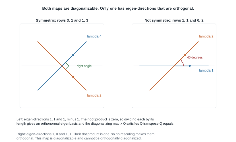
The panels show the phenomenon from both sides. On the left the symmetric matrix with rows \((3,1)\) and \((1,3)\) has eigenvalue \(4\) along \((1,1)\) and eigenvalue \(2\) along \((1,-1)\) — check by multiplying, since \((3+1, 1+3) = 4(1,1)\) and \((3-1, 1-3) = 2(1,-1)\) — and those directions meet at a right angle, so scaling each to unit length gives an orthonormal eigenbasis. On the right the matrix with rows \((1,1)\) and \((0,2)\) is diagonalizable, with eigenvalue \(1\) along \((1,0)\) and eigenvalue \(2\) along \((1,1)\), meeting at forty-five degrees; no rescaling fixes that, since rescaling does not change the line a vector spans. Diagonalizable says the eigen-directions fill the space; orthogonally diagonalizable says they also meet at right angles.

The spectral theorem and how far it reaches

The two propositions constrain eigenvalues and eigenvectors but promise none. Over \(\mathbb{R}\) nothing so far rules out a symmetric operator with no eigenvector at all, so existence has to be argued. Once it is in hand, an induction on dimension does the rest, and that induction is where finite-dimensionality earns its keep.

The induction that proves it

Lemma (existence over \(\mathbb{R}\)). Every real symmetric \(n \times n\) matrix \(A\) with \(n \ge 1\) has a real eigenvalue and a corresponding eigenvector in \(\mathbb{R}^n\).

Argument. Read \(A\) as a complex matrix on \(\mathbb{C}^n\) with the standard Hermitian inner product. The entries are real, so \(A^{*} = \overline{A}^{\mathsf{T}} = A^{\mathsf{T}} = A\), and \(A\) is Hermitian; the standard basis is orthonormal, so the operator it defines is self-adjoint. Now \(p_A(t)\) is monic of degree \(n \ge 1\), so the fundamental theorem of algebra supplies a root \(\lambda \in \mathbb{C}\), which is an eigenvalue over \(\mathbb{C}\) by the Week 10 equivalence, and the first proposition forces \(\lambda \in \mathbb{R}\). Finally \(A - \lambda I\) is a real matrix of determinant zero, and row reducing a real matrix produces the same echelon shape whether the arithmetic runs in \(\mathbb{R}\) or in \(\mathbb{C}\), so its rank agrees over both fields; its real null space therefore has positive dimension. An analytic route — maximise \(\langle Av, v \rangle\) over the unit sphere — avoids determinants entirely, at the cost of importing compactness.

Theorem (spectral theorem). Let \(V\) be a finite-dimensional inner product space over \(\mathbb{R}\) or \(\mathbb{C}\) with \(\dim V = n \ge 1\), and let \(T \in \mathcal{L}(V)\) be self-adjoint. Then \(V\) has an orthonormal basis consisting of eigenvectors of \(T\).

Argument. Induct on \(n\). If \(n = 1\) then \(Tv \in V = \operatorname{span}(v)\) for any nonzero \(v\), so \(v/\lVert v \rVert\) is the required basis. Let \(n > 1\). Gram-Schmidt supplies an orthonormal basis \(\mathcal{B}\) of \(V\), and the proposition above makes \(A = [T]_{\mathcal{B} \leftarrow \mathcal{B}}\) satisfy \(A^{*} = A\) — here orthonormality of \(\mathcal{B}\) is needed — which over \(\mathbb{R}\) says that \(A\) is symmetric. One eigenvector now has to be produced, and that is the only step at which the two fields part company. Over \(\mathbb{R}\) the lemma supplies a real eigenvalue \(\lambda\) of \(A\) together with a real eigenvector. Over \(\mathbb{C}\) the work is shorter than the lemma: \(p_A\) is monic of degree \(n \ge 1\), so the fundamental theorem of algebra gives a root \(\lambda\), the Week 10 equivalence turns it into an eigenvalue with an eigenvector in \(\mathbb{C}^n\), and the first proposition forces \(\lambda \in \mathbb{R}\). Either way, transporting that eigenvector through the coordinate isomorphism produces \(v \ne 0\) in \(V\) with \(Tv = \lambda v\) and \(\lambda\) real. Put \(e_1 = v/\lVert v \rVert\) and \(U = \operatorname{span}(e_1)\).

Now the step the proof turns on: \(U^{\perp}\) is invariant under \(T\). For \(w \in U^{\perp}\), \[\langle Tw, e_1 \rangle = \langle w, Te_1 \rangle = \langle w, \lambda e_1 \rangle = \lambda \langle w, e_1 \rangle = 0,\] using self-adjointness in the first equality and \(\lambda\) real in the third, so \(Tw \in U^{\perp}\). Week 8 gives \(V = U \oplus U^{\perp}\) with \(\dim U^{\perp} = n - 1\), and that is where finite-dimensionality is spent. The restriction \(T|_{U^{\perp}}\) is an operator on \(U^{\perp}\) with the restricted inner product, self-adjoint there because \(\langle Tw, z \rangle = \langle w, Tz \rangle\) holds for all \(w, z \in V\) and in particular inside \(U^{\perp}\). By induction \(U^{\perp}\) has an orthonormal basis \((e_2, \dots, e_n)\) of eigenvectors of \(T|_{U^{\perp}}\), which are eigenvectors of \(T\). Each lies in \(U^{\perp}\), hence is orthogonal to \(e_1\), so \((e_1, \dots, e_n)\) is an orthonormal set of \(n\) vectors, independent by Week 6 and a basis by the Week 2 dimension count.

Corollary (matrix form). A real \(n \times n\) matrix satisfies \(A^{\mathsf{T}} = A\) if and only if \(A = QDQ^{\mathsf{T}}\) for some real orthogonal \(Q\) and real diagonal \(D\); a complex one satisfies \(A^{*} = A\) if and only if \(A = UDU^{*}\) with \(U\) unitary and \(D\) real diagonal.

Argument. Forwards, apply the theorem on \(\mathbb{R}^n\) or \(\mathbb{C}^n\) with the standard inner product and let the columns of \(Q\) be the orthonormal eigenvectors. The \((i,j)\) entry of \(Q^{\mathsf{T}}Q\) is the inner product of columns \(i\) and \(j\), so \(Q^{\mathsf{T}}Q = I\) and \(Q^{-1} = Q^{\mathsf{T}}\). Column \(j\) of \(AQ\) is \(\lambda_j\) times the \(j\)-th eigenvector, which is column \(j\) of \(QD\) with \(D = \operatorname{diag}(\lambda_1, \dots, \lambda_n)\), so \(AQ = QD\) and \(Q^{\mathsf{T}}AQ = D\). Backwards, \((QDQ^{\mathsf{T}})^{\mathsf{T}} = QD^{\mathsf{T}}Q^{\mathsf{T}} = QDQ^{\mathsf{T}}\). The complex case is identical with conjugate transposes, using \(D^{*} = D\) because \(D\) is diagonal and real. The converse direction is what upgrades the theorem from an implication to a characterisation.

One word on the field, since this block insists on it. Everything above runs over \(\mathbb{R}\) or \(\mathbb{C}\) and nowhere else: positive-definiteness compares \(\langle v, v \rangle\) with zero, which needs an ordered field, so there is no inner-product theory of this kind over \(\mathbb{F}_2\). Over \(\mathbb{Q}\) the statement fails outright for want of roots. The symmetric matrix with rows \((1,1)\) and \((1,0)\) has characteristic polynomial \(t^2 - t - 1\), whose roots are irrational, so as an operator on \(\mathbb{Q}^2\) it has no eigenvalue at all, let alone an eigenbasis. Symmetry constrains where the eigenvalues live; it does not conjure them into a field too small to hold them.

Spectral decomposition as a sum of projections

The basis form is convenient for computing; the projection form is better for reasoning, because it removes the arbitrary choices made inside a repeated eigenspace.

Let \(T\) be self-adjoint on a finite-dimensional inner product space \(V\) with distinct eigenvalues \(\lambda_1, \dots, \lambda_k\). Group the orthonormal eigenbasis by eigenvalue. Each group is an orthonormal subset of \(E_{\lambda_i} = \ker(T - \lambda_i I)\), and spans it: if \(v \in E_{\lambda_i}\), expand \(v\) in the whole eigenbasis, apply \(T\), and compare coefficients; a basis vector with eigenvalue \(\mu \ne \lambda_i\) carries a coefficient \(c\) with \(\mu c = \lambda_i c\), forcing \(c = 0\). So each group is an orthonormal basis of its eigenspace, the eigenspaces are mutually orthogonal by the second proposition above, and \(V\) is their orthogonal direct sum.

Let \(P_i\) be the orthogonal projection onto \(E_{\lambda_i}\), which by Week 7 is \(P_iv = \sum_e \langle v, e \rangle e\) summed over the \(i\)-th group. Three identities follow from the expansion \(v = \sum_e \langle v, e \rangle e\) against the full orthonormal basis: \[P_1 + \dots + P_k = I, \qquad P_iP_j = 0 \ \text{ for } i \ne j, \qquad T = \lambda_1P_1 + \dots + \lambda_kP_k .\] The first is that expansion regrouped; the second holds because the ranges are orthogonal; the third comes from applying \(T\) term by term. Each \(P_i\) is self-adjoint and idempotent, which by Week 7 characterises an orthogonal projection.

The spectral decomposition of a three-by-three symmetric matrix drawn on a dimension bar.

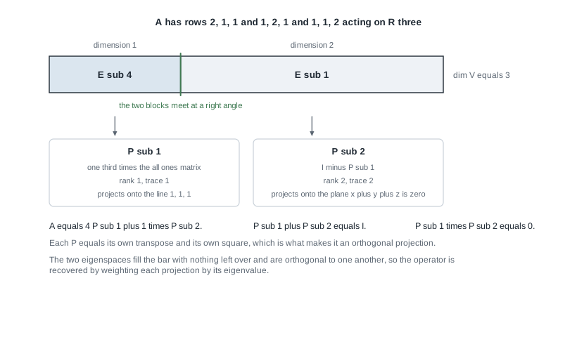
The bar shows the arithmetic of the worked example below before you compute it. The eigenspaces fill it exactly, which says the geometric multiplicities sum to \(\dim V\), and the join between the blocks is a right angle rather than an arbitrary splitting. One consequence deserves saying aloud. Since \(\sum_i \operatorname{geo}(\lambda_i) = \dim V = \sum_i \operatorname{alg}(\lambda_i)\) while \(\operatorname{geo}(\lambda) \le \operatorname{alg}(\lambda)\) always, the two multiplicities must agree at every eigenvalue of a self-adjoint operator: the Week 11 criterion is satisfied automatically and never needs checking.

Because \(P_iP_j = 0\) and \(P_i^2 = P_i\), expanding \((\sum_i \lambda_iP_i)^2\) leaves only diagonal terms, so \(T^m = \sum_i \lambda_i^mP_i\) and \(f(T) = \sum_i f(\lambda_i)P_i\) for every polynomial \(f\); and if every \(\lambda_i \ge 0\) then \(S = \sum_i \sqrt{\lambda_i}\,P_i\) is self-adjoint with \(S^2 = T\), a positive square root built from spectral data alone.

Normal operators, and the widest complex statement

Self-adjointness is sufficient for an orthonormal eigenbasis but not necessary, and over \(\mathbb{C}\) the exact condition is clean.

Definition. \(T \in \mathcal{L}(V)\) is normal when \(TT^{*} = T^{*}T\).

Self-adjoint operators are normal, since both products are \(T^2\); unitary ones are normal, since both are \(I\). The converse fails, and the failure is common rather than exotic.

Lemma. If \(T\) is normal on an inner product space \(V\), then \(\lVert Tv \rVert = \lVert T^{*}v \rVert\) for every \(v\).

Argument. \(\lVert Tv \rVert^2 = \langle Tv, Tv \rangle = \langle T^{*}Tv, v \rangle = \langle TT^{*}v, v \rangle = \langle T^{*}v, T^{*}v \rangle = \lVert T^{*}v \rVert^2\), moving \(T\) across by the defining property of the adjoint and using normality in the middle step.

Corollary. If \(T\) is normal and \(Tv = \lambda v\), then \(T^{*}v = \overline{\lambda}v\); consequently eigenvectors of a normal operator for distinct eigenvalues are orthogonal.

Argument. First \(S = T - \lambda I\) is normal, since \(SS^{*} = TT^{*} - \overline{\lambda}T - \lambda T^{*} + \lvert \lambda \rvert^2 I\) and \(S^{*}S = T^{*}T - \lambda T^{*} - \overline{\lambda}T + \lvert \lambda \rvert^2 I\) agree exactly when \(TT^{*} = T^{*}T\). Since \(S^{*} = T^{*} - \overline{\lambda}I\), the lemma gives \(\lVert S^{*}v \rVert = \lVert Sv \rVert = 0\), so \(T^{*}v = \overline{\lambda}v\). Then for \(Tu = \lambda u\) and \(Tv = \mu v\) with \(\lambda \ne \mu\), \(\lambda \langle u, v \rangle = \langle Tu, v \rangle = \langle u, T^{*}v \rangle = \langle u, \overline{\mu}v \rangle = \mu \langle u, v \rangle\).

Theorem (complex spectral theorem). Let \(V\) be a finite-dimensional complex inner product space and \(T \in \mathcal{L}(V)\). Then \(V\) has an orthonormal basis of eigenvectors of \(T\) if and only if \(T\) is normal.

Argument. If such a basis \(\mathcal{B}\) exists then \([T]_{\mathcal{B} \leftarrow \mathcal{B}} = D\) is diagonal and, \(\mathcal{B}\) being orthonormal, \([T^{*}]_{\mathcal{B} \leftarrow \mathcal{B}} = D^{*}\) is diagonal too; diagonal matrices commute, so \(TT^{*} = T^{*}T\). Conversely let \(T\) be normal and induct on \(\dim V\), the case \(\dim V = 1\) being immediate. Since \(\mathbb{C}\) is algebraically closed, \(p_T\) has a root, so there is a unit eigenvector \(e_1\) with \(Te_1 = \lambda e_1\), and the corollary gives \(T^{*}e_1 = \overline{\lambda}e_1\). Put \(U = \operatorname{span}(e_1)\). For \(w \in U^{\perp}\) both \(\langle Tw, e_1 \rangle = \langle w, T^{*}e_1 \rangle = \lambda \langle w, e_1 \rangle = 0\) and \(\langle T^{*}w, e_1 \rangle = \langle w, Te_1 \rangle = \overline{\lambda}\langle w, e_1 \rangle = 0\), so \(U^{\perp}\) is invariant under \(T\) and under \(T^{*}\). Because both restrictions land back in \(U^{\perp}\), the adjoint of \(T|_{U^{\perp}}\) computed inside \(U^{\perp}\) is \(T^{*}|_{U^{\perp}}\), and the two commute because their unrestricted versions do; so \(T|_{U^{\perp}}\) is normal on a space of dimension \(\dim V - 1\) and the induction applies. The one compressed step is that identification of the restricted adjoint, which uses both invariances and nothing else.

Self-adjoint and unitary operators drawn as overlapping classes inside the normal ones, with a non-normal example outside.

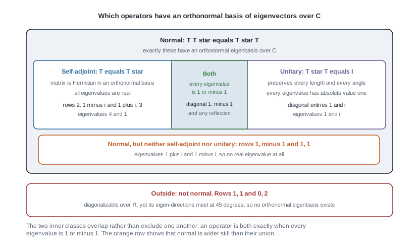
The containment picture organises the week. Inside the normal box the self-adjoint operators are those with every eigenvalue real and the unitary ones those with every eigenvalue of absolute value one; those two conditions overlap rather than exclude one another, and an operator satisfies both exactly when every eigenvalue is \(1\) or \(-1\), as the identity, any reflection, and \(\operatorname{diag}(1,-1)\) all do. The row along the bottom holds a normal matrix that is neither, developed in the second worked example. Outside sits the matrix with rows \((1,1)\) and \((0,2)\), diagonalizable over \(\mathbb{R}\) and not normal, which is why its eigen-directions were free to meet at forty-five degrees. Over \(\mathbb{R}\) the picture is less tidy: the quarter-turn \(R(x,y) = (-y,x)\) satisfies \(R^{\mathsf{T}}R = RR^{\mathsf{T}} = I\), so it is normal, yet has no real eigenvalue at all. Normality is the right condition only over an algebraically closed field; over \(\mathbb{R}\) the right condition is symmetry.

Closing the Week 9 loop: congruence meets similarity

Week 9 left an explicit promise. Congruence acts by \(M \mapsto P^{\mathsf{T}}MP\) and classifies real symmetric matrices by signature; similarity acts by \(M \mapsto P^{-1}MP\) and classifies operators by finer data including eigenvalues. On real symmetric matrices the two relations are not independent: similarity is the strictly finer one. Similar matrices share a characteristic polynomial, hence eigenvalues with multiplicity, and the paragraph below identifies the signature with the signs of those eigenvalues, so similar real symmetric matrices have equal signatures and are congruent by Sylvester’s law. The converse fails: \(\operatorname{diag}(1,1)\) and \(\operatorname{diag}(1,2)\) are congruent, both forms being positive definite, yet their eigenvalues differ, so they are not similar. The two laws coincide exactly when \(P^{\mathsf{T}} = P^{-1}\), that is, when \(P\) is orthogonal.

The spectral theorem supplies such a \(P\) for every real symmetric \(M\). Writing \(Q^{\mathsf{T}}MQ = D\) with \(Q\) orthogonal, that single equation is a similarity, so \(D\) carries the eigenvalues with their multiplicities, and a congruence, so by Sylvester’s law of inertia \(D\) carries the signature of \(q(v) = v^{\mathsf{T}}Mv\). Hence the signature of a real quadratic form is the count of positive, negative, and zero eigenvalues of its symmetric matrix. In particular \(M\) is positive definite exactly when every eigenvalue is positive — far more usable than completing the square, and the reason the leading-principal-minor test quoted in Week 9 works.

The level ellipse of a quadratic form with its principal axes along the eigenvectors.

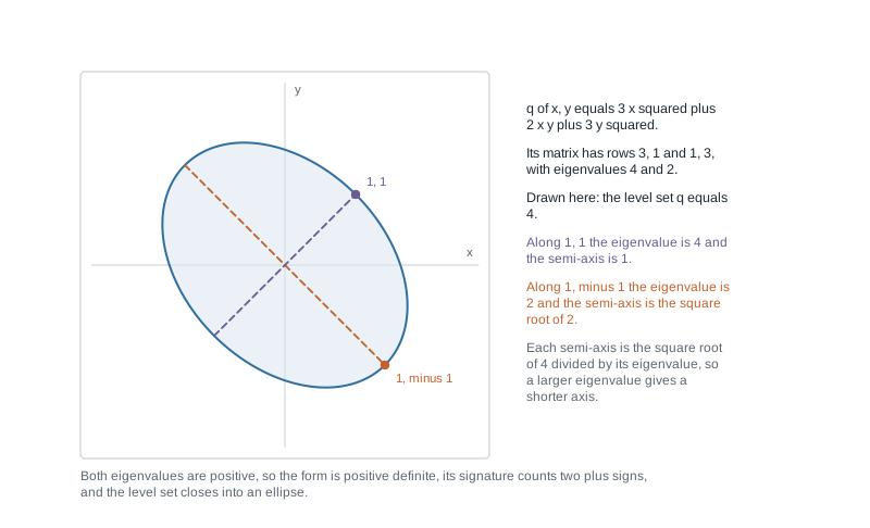
The ellipse makes the bridge visible. For \(q(x,y) = 3x^2 + 2xy + 3y^2\) the symmetric matrix has rows \((3,1)\) and \((1,3)\), with the eigenvalues \(4\) and \(2\) found above. In the orthonormal eigenbasis \(\tfrac{1}{\sqrt{2}}(1,1)\) and \(\tfrac{1}{\sqrt{2}}(1,-1)\) the form becomes \(4u^2 + 2v^2\), so the level set \(q = 4\) is \(u^2 + v^2/2 = 1\): semi-axis \(1\) along the eigenvalue-\(4\) direction and semi-axis \(\sqrt{2}\) along the eigenvalue-\(2\) direction. Each semi-axis is \(\sqrt{4/\lambda}\), so a larger eigenvalue pinches the level set closer to the origin. Check one point: \((1,-1)\) lies on the drawn curve and \(q(1,-1) = 3 - 2 + 3 = 4\). Both eigenvalues are positive, the signature counts two positive entries and none negative, and the level set is a bounded ellipse rather than a hyperbola — three ways of saying the same thing.

Worked example — orthogonally diagonalising a three-by-three real symmetric matrix

Work in \(\mathbb{R}^3\) with the dot product and the standard basis, which is orthonormal, and take \[A = \begin{pmatrix} 2 & 1 & 1 \\ 1 & 2 & 1 \\ 1 & 1 & 2 \end{pmatrix} .\] It equals its own transpose, so \(v \mapsto Av\) is self-adjoint. The task is to produce an orthogonal \(Q\) and a diagonal \(D\) with \(Q^{\mathsf{T}}AQ = D\), verifying both defining equations by multiplication.

Step 1. The characteristic polynomial. Put \(s = t - 2\), so that \[p_A(t) = \det\begin{pmatrix} s & -1 & -1 \\ -1 & s & -1 \\ -1 & -1 & s \end{pmatrix} = s(s^2 - 1) + \big({-s} - 1\big) - (1 + s) = s^3 - 3s - 2 .\] Since \(s = -1\) gives \(-1 + 3 - 2 = 0\), the factor \(s + 1\) divides it, and dividing twice gives \((s+1)^2(s-2)\). Restoring \(s = t - 2\), \[p_A(t) = (t-1)^2(t-4) = t^3 - 6t^2 + 9t - 4 .\] Two checks: the eigenvalues \(4, 1, 1\) sum to \(6 = \operatorname{tr} A\), and their product is \(4 = \det A\), confirmed by \(2(4-1) - 1(2-1) + 1(1-2) = 6 - 1 - 1 = 4\). So \(\operatorname{alg}(4) = 1\), \(\operatorname{alg}(1) = 2\), and both eigenvalues are real as promised.

Step 2. The eigenspaces. For \(\lambda = 4\) solve \((A - 4I)v = 0\): the rows read \(-2x + y + z = 0\), \(x - 2y + z = 0\), \(x + y - 2z = 0\). Subtracting the first two gives \(3x - 3y = 0\), so \(x = y\), and then the first gives \(z = x\). Hence \(E_4 = \operatorname{span}\{(1,1,1)\}\) and \(\operatorname{geo}(4) = 1\). For \(\lambda = 1\) all three rows of \(A - I\) read \(x + y + z = 0\), so \(E_1\) is that plane and \(\operatorname{geo}(1) = 2\). Both multiplicities match their algebraic counterparts, as the theorem guarantees in advance.

Step 3. Orthogonality for free, and Gram-Schmidt where it is not. Every vector of \(E_1\) is orthogonal to \((1,1,1)\), since \(x + y + z = 0\) is precisely that inner product vanishing. Inside \(E_1\) nothing is free. Take \(w_1 = (1,-1,0)\) and \(w_2 = (1,0,-1)\), both in the plane, with \(\langle w_2, w_1 \rangle = 1 \ne 0\); one Gram-Schmidt step from Week 6 gives \[w_2' = w_2 - \frac{\langle w_2, w_1 \rangle}{\langle w_1, w_1 \rangle}w_1 = (1,0,-1) - \tfrac12(1,-1,0) = \big(\tfrac12, \tfrac12, -1\big),\] and clearing the fraction gives \((1,1,-2)\), still in the plane since \(1 + 1 - 2 = 0\), and orthogonal to \(w_1\) since \(1 - 1 + 0 = 0\).

Step 4. Normalise and assemble. The three vectors have squared lengths \(3\), \(2\), \(6\), so \[q_1 = \tfrac{1}{\sqrt{3}}(1,1,1), \qquad q_2 = \tfrac{1}{\sqrt{2}}(1,-1,0), \qquad q_3 = \tfrac{1}{\sqrt{6}}(1,1,-2),\] \[Q = \begin{pmatrix} 1/\sqrt{3} & 1/\sqrt{2} & 1/\sqrt{6} \\ 1/\sqrt{3} & -1/\sqrt{2} & 1/\sqrt{6} \\ 1/\sqrt{3} & 0 & -2/\sqrt{6} \end{pmatrix}, \qquad D = \begin{pmatrix} 4 & 0 & 0 \\ 0 & 1 & 0 \\ 0 & 0 & 1 \end{pmatrix} .\]

Step 5. Verify \(Q^{\mathsf{T}}Q = I\). The diagonal entries are the squared lengths: \((1+1+1)/3 = 1\), \((1+1+0)/2 = 1\), \((1+1+4)/6 = 1\). The off-diagonal entries are the pairwise inner products: \((1 - 1 + 0)/\sqrt{6} = 0\), \((1 + 1 - 2)/\sqrt{18} = 0\), \((1 - 1 + 0)/\sqrt{12} = 0\). So \(Q^{\mathsf{T}}Q = I\) and \(Q^{-1} = Q^{\mathsf{T}}\), with no row reduction anywhere.

Step 6. Verify \(Q^{\mathsf{T}}AQ = D\). It is enough to check \(AQ = QD\) column by column. \(A(1,1,1) = (2+1+1,\, 1+2+1,\, 1+1+2) = (4,4,4) = 4(1,1,1)\); \(A(1,-1,0) = (2-1+0,\, 1-2+0,\, 1-1+0) = (1,-1,0)\); \(A(1,1,-2) = (2+1-2,\, 1+2-2,\, 1+1-4) = (1,1,-2)\). So \(AQ\) has columns \(4q_1, q_2, q_3\), which is exactly \(QD\), and multiplying on the left by \(Q^{\mathsf{T}} = Q^{-1}\) gives \(Q^{\mathsf{T}}AQ = D\).

Step 7. The projection form. With \(J\) the three-by-three matrix of all ones, \(P_1 = q_1q_1^{\mathsf{T}} = \tfrac13 J\) and \(P_2 = I - P_1\). Then \(P_1^2 = \tfrac19 J^2 = \tfrac19(3J) = \tfrac13 J = P_1\), both are symmetric, \(P_1 + P_2 = I\), and \(P_1P_2 = P_1 - P_1^2 = 0\). Finally \(4P_1 + 1 \cdot P_2 = \tfrac43 J + I - \tfrac13 J = I + J = A\), since \(A\) is \(I + J\) entry by entry. The ranks \(1\) and \(2\) match the geometric multiplicities and the dimension bar above.

What this establishes: an orthogonal change of coordinates in which \(A\) acts by scaling, and a basis-free decomposition of \(A\) into orthogonal projections. What it does not establish is that \(Q\) is unique — replacing \(q_2\) by \(-q_2\), or rotating \((q_2, q_3)\) inside the plane \(E_1\), gives another valid \(Q\); only the eigenspaces and their projections are canonical. Straight from Week 9: all three eigenvalues are positive, so \(q(v) = v^{\mathsf{T}}Av\) has signature three positive and none negative, and is positive definite.

The same reasoning, transferred

Move to \(\mathbb{C}^2\) with the standard Hermitian inner product and take \[A = \begin{pmatrix} 2 & 1 - i \\ 1 + i & 3 \end{pmatrix}, \qquad A^{*} = \overline{A}^{\mathsf{T}} = A,\] so \(A\) is Hermitian; note \(A^{\mathsf{T}} \ne A\), so the plain transpose would have given the wrong verdict. Here \(\operatorname{tr} A = 5\) and \(\det A = 6 - (1-i)(1+i) = 6 - 2 = 4\), so \(p_A(t) = t^2 - 5t + 4 = (t-1)(t-4)\) with eigenvalues \(4\) and \(1\), both real as required. For \(\lambda = 4\) the first row of \(A - 4I\) gives \(-2x + (1-i)y = 0\), so \(y = 2\) yields \(v_1 = (1-i, 2)\), and the second row checks out: \((1+i)(1-i) - 2 = 2 - 2 = 0\). For \(\lambda = 1\) the first row gives \(x + (1-i)y = 0\), so \(v_2 = (-1+i, 1)\), with \((1+i)(-1+i) + 2 = -2 + 2 = 0\). Orthogonality is automatic and worth checking: \(\langle v_1, v_2 \rangle = (1-i)\overline{(-1+i)} + 2 = (1-i)(-1-i) + 2 = -2 + 2 = 0\). Squared lengths are \(6\) and \(3\), so \[U = \begin{pmatrix} (1-i)/\sqrt{6} & (-1+i)/\sqrt{3} \\ 2/\sqrt{6} & 1/\sqrt{3} \end{pmatrix}, \qquad U^{*}AU = \begin{pmatrix} 4 & 0 \\ 0 & 1 \end{pmatrix},\] verified by \(Av_1 = (2(1-i) + 2(1-i),\; (1+i)(1-i) + 6) = (4-4i, 8) = 4v_1\) and \(Av_2 = (2(-1+i) + (1-i),\; (1+i)(-1+i) + 3) = (-1+i, 1) = v_2\).

What stayed the same: the characteristic polynomial, the eigenspace computation, the automatic orthogonality across distinct eigenvalues, and the verification by columns. What changed: conjugation enters in three places — forming \(A^{*}\), computing the inner product, and transposing \(U\) — and the entries of \(U\) are complex while \(D\) stays real, which is the eigenvalue proposition in action. The dimension changed too, and with it the Gram-Schmidt step vanished, because every eigenvalue here is simple and no repeated eigenspace needs orthogonalising.

Second worked example — a normal matrix that is neither Hermitian nor unitary

Take the real matrix \(N = \begin{pmatrix} 1 & -1 \\ 1 & 1 \end{pmatrix}\), regarded as an operator on \(\mathbb{C}^2\) with the standard Hermitian inner product. The entries are real, so \(N^{*} = N^{\mathsf{T}} = \begin{pmatrix} 1 & 1 \\ -1 & 1 \end{pmatrix}\).

Step 1. Normal, and neither special case. Multiply both ways: \(NN^{*} = \begin{pmatrix} 1+1 & 1-1 \\ 1-1 & 1+1 \end{pmatrix} = 2I\) and \(N^{*}N = \begin{pmatrix} 1+1 & -1+1 \\ -1+1 & 1+1 \end{pmatrix} = 2I\), so \(N\) is normal. It is not self-adjoint, the entries above and below the diagonal differing in sign, and not unitary, since \(N^{*}N = 2I \ne I\). Geometrically \(N = \sqrt{2}\,R\) with \(R\) the rotation by an eighth of a turn: the rotation breaks self-adjointness, the scaling breaks unitarity.

Step 2. Over \(\mathbb{R}\) there is nothing to find. Here \(p_N(t) = t^2 - 2t + 2\), whose discriminant is \(4 - 8 = -4\), negative, so there is no real root, no real eigenvalue, and no invariant line in \(\mathbb{R}^2\). This is the field failure the block keeps in its pocket, and it is why the real theorem is stated for symmetric operators and not for normal ones.

Step 3. Over \(\mathbb{C}\) the eigenvalues appear as a conjugate pair. The roots are \(t = 1 \pm i\). For \(\lambda = 1+i\) the first row of \(N - (1+i)I\) reads \(-ix - y = 0\), so \(v_1 = (1, -i)\), confirmed by the second row, \(1 \cdot 1 + (-i)(-i) = 1 - 1 = 0\). For \(\lambda = 1-i\) the first row reads \(ix - y = 0\), so \(v_2 = (1, i)\), with \(1 + i \cdot i = 0\). Both eigenvalues are non-real, exactly as the theory allows once \(T\) is normal without being self-adjoint.

Step 4. Orthogonality and the unitary matrix. Compute \(\langle v_1, v_2 \rangle = 1 \cdot \overline{1} + (-i)\overline{i} = 1 + (-i)(-i) = 1 - 1 = 0\), as the corollary for normal operators promised. Each has squared length \(2\), so \[U = \tfrac{1}{\sqrt{2}}\begin{pmatrix} 1 & 1 \\ -i & i \end{pmatrix}, \qquad U^{*} = \tfrac{1}{\sqrt{2}}\begin{pmatrix} 1 & i \\ 1 & -i \end{pmatrix}, \qquad D = \begin{pmatrix} 1+i & 0 \\ 0 & 1-i \end{pmatrix}.\] Check \(U^{*}U = I\) entry by entry: \(\tfrac12(1 + i(-i)) = 1\), \(\tfrac12(1 + i \cdot i) = 0\), \(\tfrac12(1 + (-i)(-i)) = 0\), \(\tfrac12(1 + (-i)i) = 1\).

Step 5. Verify \(U^{*}NU = D\). Check \(NU = UD\) by columns. First, \(N(1,-i) = (1 + i,\; 1 - i)\), while \((1+i)(1,-i) = (1+i,\; -i - i^2) = (1+i,\; 1-i)\). Second, \(N(1,i) = (1 - i,\; 1 + i)\), while \((1-i)(1,i) = (1-i,\; i - i^2) = (1-i,\; 1+i)\). Both agree, so \(NU = UD\) and, multiplying on the left by \(U^{*} = U^{-1}\), \(U^{*}NU = D\).

Step 6. What this shows and what it does not. The complex spectral theorem is genuinely wider than the Hermitian case: \(N\) has an orthonormal eigenbasis with no real eigenvalue in sight, and no real orthogonal conjugation could have diagonalised it, since \(Q^{\mathsf{T}}NQ\) is symmetric only when \(N\) is. It does not show normality suffices over \(\mathbb{R}\) — Step 2 refutes that. Nor are the eigenvalues arbitrary: \(\lvert 1 \pm i \rvert = \sqrt{2}\), so \(N/\sqrt{2}\) is unitary with both eigenvalues on the unit circle.

The misreading to avoid

The misreading runs like this: symmetric matrices are diagonalizable over \(\mathbb{R}\), and diagonalizable is the property that matters, so any diagonalizable real matrix can be orthogonally diagonalised. The first clause is true and this week proved it; the last is false, and the counterexample has already appeared twice. The matrix with rows \((1,1)\) and \((0,2)\) has distinct eigenvalues \(1\) and \(2\), hence is diagonalizable by the Week 11 sufficient condition, with eigenvectors \((1,0)\) and \((1,1)\). Their inner product is \(1\) and the angle between them is forty-five degrees, so they cannot be rescaled into an orthonormal pair; any \(P\) diagonalising the matrix has non-orthogonal columns and \(P^{-1} \ne P^{\mathsf{T}}\).

What makes the refutation airtight is the converse half of the corollary. If \(A = QDQ^{\mathsf{T}}\) with \(Q\) real orthogonal and \(D\) real diagonal, then \(A^{\mathsf{T}} = QD^{\mathsf{T}}Q^{\mathsf{T}} = QDQ^{\mathsf{T}} = A\), so \(A\) is symmetric. Orthogonal diagonalizability therefore implies symmetry, the spectral theorem is an equivalence rather than a one-way street, and since the matrix above is not symmetric no orthogonal \(Q\) can diagonalise it. Diagonalizable and orthogonally diagonalizable are different properties, with the second strictly stronger over \(\mathbb{R}\) and equivalent to symmetry.

A second misreading is quieter and does more damage: my basis is a basis of eigenvectors, so I can expand vectors and build projections with inner products. Week 6’s expansion and Week 7’s projection formula both require the \(e_i\) to be orthonormal, not merely a basis; the failed computation in the motivation section returned \((\tfrac12, \tfrac12)\) where the vector was \((0,1)\). A third, narrower slip: in a non-orthonormal basis a symmetric matrix is no certificate of self-adjointness and an unsymmetric one no refutation — the self-adjoint \(T(x,y) = (3x+y, x+3y)\) has the unsymmetric matrix with rows \((2,0)\) and \((1,4)\) in the basis \((1,0), (1,1)\).

Practice on your own

These are for your own checking rather than for submission, and each is within reach of Weeks 5 through 12.

1. A vanishing form. Let \(V\) be a finite-dimensional real inner product space and \(T \in \mathcal{L}(V)\) self-adjoint with \(\langle Tv, v \rangle = 0\) for every \(v\). Prove \(T = 0\) by expanding \(\langle T(u+v), u+v \rangle\). Then show the conclusion fails without self-adjointness: for the quarter-turn \(R(x,y) = (-y,x)\) on \(\mathbb{R}^2\), compute \(\langle Rv, v \rangle\) for general \(v\) and observe that it vanishes identically while \(R \ne 0\).
2. A two-by-two orthogonal diagonalisation. Orthogonally diagonalise \(M\) with rows \((5,-2)\) and \((-2,2)\): find \(p_M(t)\), both eigenvalues, an orthonormal eigenbasis, and \(Q\), then verify \(Q^{\mathsf{T}}Q = I\) and \(Q^{\mathsf{T}}MQ = D\). State the signature of \(q(x,y) = 5x^2 - 4xy + 2y^2\) and the shape of the level set \(q = 1\).
3. Normal, and which kind. Let \(T\) be normal on a finite-dimensional complex inner product space. Prove that \(T\) is self-adjoint if and only if every eigenvalue is real, and unitary if and only if every eigenvalue has absolute value one. Use the orthonormal eigenbasis, and say where the argument breaks over \(\mathbb{R}\).
4. Build the trap yourself. Construct a self-adjoint operator on \(\mathbb{R}^3\) and a non-orthonormal ordered basis in which its matrix is not symmetric. Then explain in one sentence each why this does not contradict the proposition on matrices of self-adjoint operators, and why the eigenvalues computed from that unsymmetric array are nonetheless still real.
5. Commuting self-adjoint operators. Let \(S\) and \(T\) be self-adjoint on a finite-dimensional real inner product space with \(ST = TS\), and suppose \(S\) has \(\dim V\) distinct eigenvalues. Prove every eigenspace of \(S\) is invariant under \(T\), and conclude that one orthonormal basis diagonalises both. Then say what must be added when \(S\) has a repeated eigenvalue.

Where to read more

This page is self-contained, but a second treatment in another voice often settles a theorem. The three addresses below are offered online at no cost by their providers; availability and licence terms are as those providers state them, and neither is confirmed here.

• MIT OpenCourseWare 18.700 Linear Algebra — a proof-based course whose treatment of self-adjoint operators and the spectral theorem follows the induction used above.
• Linear Algebra Done Wrong by Sergei Treil — an abstract-first text covering normal operators and the spectral decomposition in this order.
• MIT OpenCourseWare 18.06 Linear Algebra — the computational complement, for symmetric matrices, positive definiteness, and the principal-axis picture on explicit arrays.
• The optional Roman alignment for this week is the chapter on eigenvalues and eigenvectors, in the sections on symmetric matrices, on Hermitian matrices, and on the spectral theorem. That text is an optional reference: a borrowed or library copy suffices, purchase is never required, and nothing from it is reproduced here.
• Course pages: the notes overview, the syllabus, the schedule, and the resources page. The learning management system remains authoritative for section logistics and graded details.

Where this goes next

This week found the operators for which diagonalization never fails and for which the diagonalizing matrix inverts by transposition, and it closed the loop Week 9 opened: along an orthogonal change of basis congruence and similarity agree, so the signature of a real quadratic form is read off the signs of the eigenvalues. What remains open is the general operator, the one with a defective eigenvalue and no orthonormal eigenbasis available at any price.

Week 13, on Schur triangularization, the minimal polynomial, and the Cayley-Hamilton theorem, takes that case up. Schur’s theorem shows every operator on a finite-dimensional complex inner product space is unitarily similar to an upper triangular matrix — orthonormality retained, diagonality surrendered — and the spectral theorem drops out of it in two lines as a check on both. The minimal polynomial \(m_T(t)\) then arrives as the invariant deciding diagonalizability outright, and Weeks 14 and 15 use it to build the Jordan canonical form. To look back: Week 11 carries the multiplicity criterion this week automatically satisfies, Week 8 carries the adjoint and the orthogonal-complement decomposition the proof rests on, and the notes index and course home page list what is here.