Week 13 — Schur triangularization, the minimal polynomial, and Cayley-Hamilton
Where this week starts
Week 11 handed you a criterion with a warning attached. An operator \(T\) on a finite-dimensional space \(V\) over \(F\) is diagonalizable exactly when its eigenspaces together fill \(V\), and plenty of operators fail that: the geometric multiplicity \(\operatorname{geo}(\lambda) = \dim E_{\lambda}\) can fall short of the algebraic multiplicity \(\operatorname{alg}(\lambda)\), and when it does, no basis of eigenvectors exists. Week 12 then found the class where failure never happens — self-adjoint operators on a finite-dimensional inner product space — using the geometry built in Weeks 5 through 9 rather than any factorisation trick.
Between those results sits every operator that is neither, and this week is about that middle. First we push the general case as far as it goes without new machinery: over \(\mathbb{C}\), every operator on a finite-dimensional inner product space is unitarily similar to an upper triangular matrix. That is Schur’s theorem. Diagonal is unavailable in general; triangular is always available, and available in an orthonormal basis, with the eigenvalues down the diagonal and every obstruction pushed above it.
Second comes the object that decides the rest of the course. Feed an operator into a polynomial and you get another operator; the polynomials sending \(T\) to zero form a family generated by one monic polynomial of least degree, the minimal polynomial \(m_T\). Two theorems follow. Cayley-Hamilton says \(p_T\) is one of those annihilating polynomials, so \(m_T\) divides \(p_T\) and \(\deg m_T \le \dim V\). And \(T\) is diagonalizable exactly when \(m_T\) factors into distinct linear factors over \(F\) — a test that reads one polynomial instead of counting eigenspace dimensions.
Three habits should be in place by the end. When an operator resists diagonalization, reach for a triangular form. When you want to know what an operator satisfies, compute \(m_T\) rather than \(p_T\). And when two matrices share a characteristic polynomial, do not conclude they are the same operator in disguise: this page exhibits the counterexample, and Weeks 14 and 15 close the gap.
Why this matters beyond the definition
Here is a claim that gets made and is false: the characteristic polynomial determines the operator up to similarity. It sounds plausible: \(p_T\) is a similarity invariant, it encodes the eigenvalues with their algebraic multiplicities, and for a \(2 \times 2\) matrix with two distinct roots it really does settle everything. But take \(D = \begin{pmatrix} 2 & 0 \\ 0 & 2 \end{pmatrix}\) and \(J = \begin{pmatrix} 2 & 1 \\ 0 & 2 \end{pmatrix}\). Both have \(p(t) = (t-2)^2\). They are not similar: \(P^{-1}DP = 2I\) for every invertible \(P\), since \(D\) is a scalar multiple of the identity, while \(J \ne 2I\). The minimal polynomials separate them at once, \(m_D(t) = t - 2\) against \(m_J(t) = (t-2)^2\).
The second stake is computational. Much of applied linear algebra runs on the fact that \(A^{-1}\), \(A^{100}\), and \(e^{A}\) are combinations of finitely many powers of \(A\), and the bound on how many is \(\deg m_T\), not \(\deg p_T\) and certainly not \(n^2\). When a \(3 \times 3\) matrix satisfies a quadratic relation, every polynomial in \(A\) collapses to the form \(aA + bI\), and knowing that in advance saves the work rather than repeating it.
What you will be able to do
- State Schur’s theorem with its hypotheses — a finite-dimensional inner product space over \(\mathbb{C}\) — and prove it by induction on the dimension using an invariant orthogonal complement.
- Derive the spectral theorem for a self-adjoint operator from a Schur form in two lines, and say which hypothesis does the work.
- Prove that the minimal polynomial exists, is unique, and divides every polynomial that annihilates the operator.
- Prove the Cayley-Hamilton theorem over \(\mathbb{C}\) from a Schur form, and explain precisely why substituting the matrix into \(\det(tI - A)\) is not a proof.
- Compute \(p_T\) and \(m_T\) for an explicit small matrix, decide diagonalizability from \(m_T\), and exhibit an operator where the two polynomials differ.
- Use an annihilating polynomial to express \(A^{-1}\) as a polynomial in \(A\), and verify the expression by multiplication.
Terms and notation worth fixing
| Symbol or term | What it means on this page |
|---|---|
| \(p_T(t) = \det(tI - T)\) | the characteristic polynomial, monic, in the variable \(t\); degree \(\dim V\) |
| \(m_T(t)\) | the minimal polynomial: the monic polynomial of least degree with \(m_T(T) = 0\) |
| \(f(T)\) | for \(f(t) = \sum_k c_k t^k\), the operator \(\sum_k c_k T^k\), with \(T^0 = I\) |
| annihilating polynomial | any \(f \ne 0\) in \(F[t]\) with \(f(T) = 0\); the zero here is the zero operator |
| unitarily similar | \(B = U^{*}AU\) with \(U\) unitary, so \(U^{*} = U^{-1}\); over \(\mathbb{R}\), orthogonally similar |
| Schur form | an upper triangular \(R\) with \(R = U^{*}AU\) for some unitary \(U\) |
| \(\operatorname{alg}(\lambda)\), \(\operatorname{geo}(\lambda)\) | the multiplicity of \(\lambda\) as a root of \(p_T\), and \(\dim E_{\lambda}\) |
| \(F[t]\) | polynomials in one variable over \(F\), with division with remainder available |
Triangular in an orthonormal basis
Diagonalizing an operator means finding a basis on which it acts by scalars. That is asking a lot, and Week 11 showed how it can fail. Triangularizing asks for less: a basis in which \(T\) sends each basis vector into the span of that vector and the ones before it. The demand is a nested chain of invariant subspaces rather than a full set of one-dimensional ones, and over \(\mathbb{C}\) such a chain always exists. Schur’s theorem says more: the chain can be taken orthogonal, so the change of basis is unitary.
The invariant complement that makes the induction work
Fix the hypotheses and keep them in view: \(V\) is a finite-dimensional inner product space over \(\mathbb{C}\) with \(\dim V = n \ge 1\), and \(T \in \mathcal{L}(V)\). Both are load-bearing. Finite-dimensionality gives an adjoint \(T^{*}\) and an orthogonal decomposition \(V = U \oplus U^{\perp}\) for every subspace \(U\), both from Week 8. Algebraic closure of \(\mathbb{C}\) gives eigenvalues at all: \(p_{T}\) has a root, so \(T\) has an eigenvector — Week 10, and it fails over \(\mathbb{R}\).
Theorem (Schur). Let \(V\) be a finite-dimensional inner product space over \(\mathbb{C}\) and \(T \in \mathcal{L}(V)\). Then \(V\) has an orthonormal basis \(\mathcal{B} = (u_1, \dots, u_n)\) with \([T]_{\mathcal{B} \leftarrow \mathcal{B}}\) upper triangular. Equivalently, for every \(A \in M_n(\mathbb{C})\) there is a unitary \(U\) with \(U^{*}AU\) upper triangular.
Argument. Induct on \(n = \dim V\). For \(n = 1\) every \(1 \times 1\) array is upper triangular and any unit vector is an orthonormal basis. Suppose \(n \ge 2\) and the statement holds in dimension \(n - 1\). The operator \(T^{*}\) exists because \(V\) is a finite-dimensional inner product space, and \(p_{T^{*}}\) has a root \(\mu\) in \(\mathbb{C}\), so there is a unit vector \(u\) with \(T^{*}u = \mu u\).
Let \(X = \{u\}^{\perp}\), of dimension \(n - 1\) by Week 8. Claim: \(X\) is invariant under \(T\) — note, under \(T\), not under \(T^{*}\). For \(x \in X\), \[\langle Tx, u \rangle = \langle x, T^{*}u \rangle = \langle x, \mu u \rangle = \overline{\mu}\,\langle x, u \rangle = 0 ,\] using the Week 5 convention that the inner product is conjugate-linear in its second slot. So \(Tx \in X\), and \(T|_{X}\) is an operator on \(X\), itself a finite-dimensional complex inner product space of dimension \(n-1\). The inductive hypothesis supplies an orthonormal basis \((u_1, \dots, u_{n-1})\) of \(X\) in which \(T|_{X}\) is upper triangular.
Set \(u_n = u\). Since \(u\) is a unit vector orthogonal to every member of a basis of \(X\), the list \((u_1, \dots, u_{n-1}, u_n)\) is orthonormal, and \(n\) orthonormal vectors in an \(n\)-dimensional space form a basis. Read off the matrix. For \(j \le n-1\) we have \(Tu_j \in X\) with an expansion in \(u_1, \dots, u_{n-1}\) that is upper triangular by construction, so column \(j\) has zeros below row \(j\) and a zero in row \(n\); and an upper triangular matrix places no constraint on its last column, which is \([Tu_n]_{\mathcal{B}}\). Hence the whole matrix is upper triangular. For the matrix form, let \(U\) have columns \(u_1, \dots, u_n\) written in the standard basis; it is unitary because its columns are orthonormal.
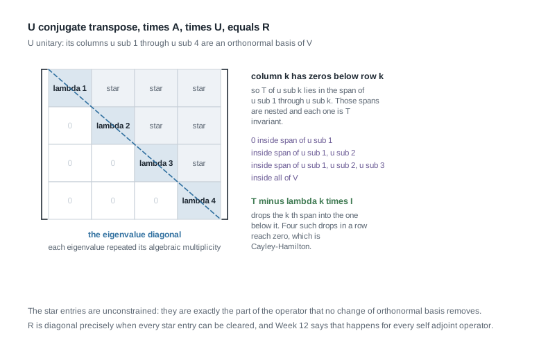
The picture records what triangularity buys. Reading column \(k\): the zeros below row \(k\) say exactly that \(Tu_k\) lies in \(\operatorname{span}(u_1, \dots, u_k)\), so those \(n\) spans form a chain of \(T\)-invariant subspaces, each one dimension larger than the last. The star entries above the diagonal are the residue no orthonormal change of basis can remove. Both features return below — the diagonal right now, the chain in the proof of Cayley-Hamilton.
What the diagonal of a Schur form records
Similar matrices have the same characteristic polynomial — Week 11 proved it, from \(\det(tI - P^{-1}AP) = \det(P^{-1}(tI - A)P) = \det(tI - A)\). So if \(R = U^{*}AU\) is upper triangular with diagonal \(r_{11}, \dots, r_{nn}\), then \(tI - R\) is upper triangular with diagonal \(t - r_{11}, \dots, t - r_{nn}\), and the determinant of a triangular matrix is the product of its diagonal entries, a fact carried over from MATH 3312. Hence \[p_A(t) = p_R(t) = \prod_{i=1}^{n} (t - r_{ii}) .\] The diagonal of a Schur form is the list of eigenvalues of \(A\), each repeated its algebraic multiplicity, in whatever order the induction produced. The order is not canonical — running the proof with a different eigenvector of \(T^{*}\) generally permutes it — but the multiset is. One consequence worth naming: \(\operatorname{tr} A\) is the sum of the eigenvalues with multiplicity and \(\det A\) their product, since both are similarity invariants read straight off \(R\). Nothing here assumed \(A\) diagonalizable.
The spectral theorem in two lines
The check that Schur is the right generalisation is that Week 12 falls out of it. Let \(A \in M_n(\mathbb{C})\) be Hermitian, meaning \(A^{*} = A\), and take a Schur form \(R = U^{*}AU\) with \(U\) unitary. Then \[R^{*} = (U^{*}AU)^{*} = U^{*}A^{*}U = U^{*}AU = R .\] So \(R\) equals its own conjugate transpose. But \(R\) is upper triangular, so \(R^{*}\) is lower triangular, and a matrix that is both is diagonal; its diagonal entries satisfy \(\overline{r_{ii}} = r_{ii}\), so they are real. That is the complex spectral theorem: a Hermitian matrix is unitarily diagonalizable with real eigenvalues, and the columns of \(U\) are an orthonormal basis of eigenvectors. The same two lines run for a normal matrix, \(AA^{*} = A^{*}A\), since a normal upper triangular matrix is diagonal — compare the \((1,1)\) entries of \(RR^{*}\) and \(R^{*}R\) and induct.
Note where the hypotheses bite. Over \(\mathbb{R}\), Schur’s theorem is false as stated: the quarter turn \(\begin{pmatrix} 0 & -1 \\ 1 & 0 \end{pmatrix}\) is not similar to any real upper triangular matrix, because such a matrix has its diagonal entries as real eigenvalues and this one has none. Symmetry rescues the real case, and that is exactly the hypothesis Week 12 carried.
The polynomials that annihilate an operator
Fix a finite-dimensional nonzero \(V\) over any field \(F\) and \(T \in \mathcal{L}(V)\). For \(f(t) = c_d t^d + \dots + c_1 t + c_0\) in \(F[t]\), write \(f(T) = c_d T^d + \dots + c_1 T + c_0 I\), with the constant term multiplied by the identity because an operator cannot be added to a scalar. Evaluation at \(T\) respects sums and products: \((f + g)(T) = f(T) + g(T)\) and \((fg)(T) = f(T)\,g(T)\), the second because powers of \(T\) commute, so the product of two polynomials in \(T\) collects exactly as it does in \(F[t]\). That consequence gets used constantly below: any two polynomials in the same \(T\) commute.
Existence, uniqueness, and division with remainder
Proposition. If \(\dim V = n\) is finite and \(V \ne \{0\}\), some nonzero \(f \in F[t]\) has \(f(T) = 0\).
Argument. By Week 4, \(\mathcal{L}(V)\) is a vector space over \(F\) of dimension \(n^2\), which is finite. The \(n^2 + 1\) operators \(I, T, T^2, \dots, T^{n^2}\) therefore cannot be linearly independent, so some nontrivial combination \(\sum_{k=0}^{n^2} c_k T^k\) is the zero operator, and \(f(t) = \sum_k c_k t^k\) annihilates \(T\). Nothing here needs algebraic closure or an inner product; it needs finite dimension, and it fails on \(F^{\mathbb{N}}\), where the shift satisfies no polynomial relation at all.
Definition. The minimal polynomial \(m_T\) is the monic polynomial of least degree with \(m_T(T) = 0\). It exists: the proposition gives an annihilating polynomial, dividing by its leading coefficient makes it monic, and the degrees of monic annihilating polynomials form a nonempty set of positive integers.
Proposition (uniqueness and divisibility). \(m_T\) is unique, and \(f(T) = 0\) if and only if \(m_T\) divides \(f\) in \(F[t]\).
Argument. Suppose \(m_1\) and \(m_2\) are monic annihilating polynomials of the least degree \(d\). Then \(m_1 - m_2\) annihilates \(T\) and has degree at most \(d - 1\), the leading terms having cancelled. If it were nonzero, dividing by its leading coefficient would produce a monic annihilating polynomial of degree less than \(d\), contradicting minimality. So \(m_1 = m_2\).
For the second claim, one direction is immediate: if \(f = q\,m_T\) then \(f(T) = q(T)\,m_T(T) = 0\). Conversely suppose \(f(T) = 0\). Division with remainder in \(F[t]\) — available over any field, since the divisor \(m_T\) is monic — gives \(f = q\,m_T + r\) with \(r = 0\) or \(\deg r < \deg m_T\). Evaluate at \(T\): \(0 = f(T) = q(T)m_T(T) + r(T) = r(T)\). If \(r \ne 0\), scaling it monic contradicts the minimality of \(\deg m_T\). So \(r = 0\) and \(m_T \mid f\).
That proposition is the reason \(m_T\) deserves a name. The annihilating polynomials are not a random collection; they are everything divisible by one generator, so checking whether \(T\) satisfies a relation becomes polynomial arithmetic rather than operator arithmetic.
Cayley-Hamilton, proved from a Schur form
Theorem (Cayley-Hamilton). Let \(V\) be a finite-dimensional nonzero space over \(\mathbb{C}\) and \(T \in \mathcal{L}(V)\). Then \(p_T(T) = 0\), the zero operator.
Argument. Put an inner product on \(V\) by declaring some basis orthonormal, which we may do because \(V\) is finite-dimensional, and take an orthonormal basis \((u_1, \dots, u_n)\) from Schur’s theorem, so the matrix of \(T\) is upper triangular with diagonal \(\lambda_1, \dots, \lambda_n\) and \(p_T(t) = (t - \lambda_1)\cdots(t - \lambda_n)\). Write \(U_k = \operatorname{span}(u_1, \dots, u_k)\) for \(k \ge 1\) and \(U_0 = \{0\}\).
The first step is a containment. Triangularity says \(Tu_k = \lambda_k u_k + w\) with \(w \in U_{k-1}\), so \((T - \lambda_k I)u_k \in U_{k-1}\), while for \(j < k\) we have \((T - \lambda_k I)u_j \in U_j \subseteq U_{k-1}\). Since \(U_k\) is spanned by \(u_1, \dots, u_k\), \[(T - \lambda_k I)\,U_k \subseteq U_{k-1} \qquad \text{for } k = 1, \dots, n .\] Now set \(Q_k = (T - \lambda_1 I)(T - \lambda_2 I)\cdots(T - \lambda_k I)\) and prove \(Q_k U_k = \{0\}\) by induction on \(k\). For \(k = 1\), \(Q_1 U_1 \subseteq U_0 = \{0\}\). For the step, \(Q_k = Q_{k-1}(T - \lambda_k I)\), and applying it to a vector of \(U_k\) first lands in \(U_{k-1}\) by the containment and then in \(\{0\}\) by the inductive hypothesis. Taking \(k = n\) gives \(Q_n V = Q_n U_n = \{0\}\), and \(Q_n = p_T(T)\) because the factors commute and their product expands to \(p_T\) evaluated at \(T\).
The picture above is this proof: the four nested spans are the \(U_k\), and each factor \(T - \lambda_k I\) steps one rung down the chain. Four steps from the top reach \(\{0\}\), which is why the product of all \(n\) factors is the zero operator and why the degree of the relation is \(n\) and not more.
Two remarks on hypotheses. Over a general field \(F\) the statement \(p_A(A) = 0\) still holds: pass to a splitting field of \(p_A\), run the argument there, and note that the entries of \(p_A(A)\) are computed by the same arithmetic in \(F\) as in the larger field, so a matrix that is zero there was zero already. Existence of a splitting field is the one thing this page quotes from algebra rather than proving. And the theorem sharpens the crude bound above: since \(m_T\) divides \(p_T\), \(\deg m_T \le n\) rather than \(n^2\).
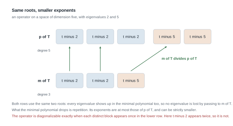
The two rows show the whole relationship. Both use the same roots — every eigenvalue of \(T\) appears in \(m_T\), proved next — and the lower row drops repetitions, never a root. Read the other way, the figure is the diagonalizability test: the operator is diagonalizable exactly when the lower row uses each distinct block once, and here \(t - 2\) appears twice, so it is not.
The test for diagonalizability
Proposition. \(m_T\) and \(p_T\) have the same roots in \(F\).
Argument. Cayley-Hamilton and divisibility give \(m_T \mid p_T\), so every root of \(m_T\) is a root of \(p_T\). Conversely let \(\lambda \in F\) be a root of \(p_T\). Then \(\det(\lambda I - T) = 0\), so \(T - \lambda I\) is not injective and there is \(v \ne 0\) with \(Tv = \lambda v\). For any \(f\), induction on the degree gives \(f(T)v = f(\lambda)v\); applied to \(m_T\) this reads \(0 = m_T(T)v = m_T(\lambda)v\), and \(v \ne 0\) forces \(m_T(\lambda) = 0\). Over a splitting field the same argument shows \(m_T\) and \(p_T\) share their irreducible factors, though not their exponents.
Theorem (diagonalizability test). Let \(V\) be finite-dimensional and nonzero over \(F\) and \(T \in \mathcal{L}(V)\). Then \(T\) is diagonalizable if and only if \(m_T(t) = (t - \lambda_1)\cdots(t - \lambda_k)\) for distinct \(\lambda_1, \dots, \lambda_k \in F\).
Argument, forward. Suppose \(T\) is diagonalizable with distinct eigenvalues \(\lambda_1, \dots, \lambda_k\), and put \(g(t) = (t - \lambda_1)\cdots(t - \lambda_k)\). Let \(v\) be a member of an eigenbasis, say \(Tv = \lambda_j v\). The factors of \(g(T)\) commute, so apply \((T - \lambda_j I)\) first; it kills \(v\). Hence \(g(T)\) vanishes on a basis, so \(g(T) = 0\) and \(m_T \mid g\). The previous proposition makes each \(\lambda_i\) a root of \(m_T\), and \(g\) has no repeated roots, so \(m_T = g\).
Argument, backward. Suppose \(m_T = (t - \lambda_1)\cdots(t - \lambda_k)\) with the \(\lambda_i\) distinct in \(F\). Define the Lagrange polynomials \[h_i(t) = \prod_{j \ne i} \frac{t - \lambda_j}{\lambda_i - \lambda_j}, \qquad i = 1, \dots, k ,\] which make sense in any field because \(\lambda_i - \lambda_j \ne 0\) for \(i \ne j\). The polynomial \(h_1 + \dots + h_k - 1\) has degree at most \(k - 1\) and vanishes at each of the \(k\) distinct scalars \(\lambda_1, \dots, \lambda_k\), since \(h_i(\lambda_i) = 1\) and \(h_i(\lambda_j) = 0\) for \(j \ne i\); but a nonzero polynomial of degree at most \(k-1\) has at most \(k-1\) roots, so it is zero. Evaluating at \(T\) gives \(h_1(T) + \dots + h_k(T) = I\), hence \(v = \sum_i h_i(T)v\) for every \(v \in V\). Moreover \[(T - \lambda_i I)\,h_i(T) = \Big(\prod_{j \ne i}(\lambda_i - \lambda_j)\Big)^{-1} m_T(T) = 0 ,\] so \(h_i(T)v \in E_{\lambda_i}\). Therefore \(V = E_{\lambda_1} + \dots + E_{\lambda_k}\); that sum is direct by Week 11, and bases of the eigenspaces strung together give an eigenbasis.
The test can fail in two genuinely different ways. The minimal polynomial may split into linear factors over \(F\) but repeat one — the defective case, and Week 11’s example with \(m_T(t) = (t-2)^2\) is exactly it. Or \(m_T\) may fail to split at all: over \(\mathbb{R}\) the quarter turn has the irreducible \(m_T(t) = t^2 + 1\), so it is not diagonalizable there; read over \(\mathbb{C}\) the same matrix has \(m_T(t) = (t - i)(t + i)\), distinct linear factors, so it is. The operator did not change. The field did.
Characteristic matters too, and \(\mathbb{F}_2\) is where you see it. Let \(A = \begin{pmatrix} 1 & 1 \\ 0 & 1 \end{pmatrix}\) over \(\mathbb{F}_2\). Then \(A^2 = \begin{pmatrix} 1 & 2 \\ 0 & 1 \end{pmatrix} = I\), so \(t^2 - 1\) annihilates \(A\). Over any field of characteristic other than two, the relation \(A^2 = I\) settles diagonalizability at once, since \(t^2 - 1 = (t-1)(t+1)\) has distinct roots there. Over \(\mathbb{F}_2\), however, \(-1 = 1\) and \(t^2 - 1 = (t-1)^2\); indeed \(m_A(t) = (t-1)^2\) here, because \(A \ne I\). And the relation itself is a consequence of \(2 = 0\), so it does not survive the change of field: read over \(\mathbb{Q}\) the same array has \(A^2 = \begin{pmatrix} 1 & 2 \\ 0 & 1 \end{pmatrix} \ne I\) and \(m_A(t) = (t-1)^2\) there too, still not diagonalizable. Over a field of characteristic other than two every involution is diagonalizable; in characteristic two the guarantee is lost — some involutions, such as the identity, are still diagonal, and some, such as this \(A\), are not.
Worked example — the characteristic and minimal polynomials of a three by three matrix
Work over \(\mathbb{Q}\) with \(V = \mathbb{Q}^3\) and the operator given in the standard basis by \[A = \begin{pmatrix} 2 & -1 & 1 \\ 1 & 1 & 0 \\ 1 & -1 & 2 \end{pmatrix} .\] The task: compute \(p_A\), determine \(m_A\) by testing the candidate divisors against the matrix, decide diagonalizability, and verify Cayley-Hamilton by multiplying out.
Step 1. The characteristic polynomial. For a \(3 \times 3\) matrix, \(p_A(t) = t^3 - (\operatorname{tr} A)t^2 + \sigma_2 t - \det A\), where \(\sigma_2\) is the sum of the three principal \(2 \times 2\) minors. Here \(\operatorname{tr} A = 2 + 1 + 2 = 5\). The principal minors are \(\det \begin{pmatrix} 1 & 0 \\ -1 & 2 \end{pmatrix} = 2\), \(\det \begin{pmatrix} 2 & 1 \\ 1 & 2 \end{pmatrix} = 3\), and \(\det \begin{pmatrix} 2 & -1 \\ 1 & 1 \end{pmatrix} = 3\), so \(\sigma_2 = 8\). Expanding along the first row, \(\det A = 2(2 - 0) + 1(2 - 0) + 1(-1 - 1) = 4 + 2 - 2 = 4\). Hence \[p_A(t) = t^3 - 5t^2 + 8t - 4 .\] Test \(t = 1\): \(1 - 5 + 8 - 4 = 0\). Divide out and factor the quadratic: \(p_A(t) = (t-1)(t^2 - 4t + 4) = (t-1)(t-2)^2\). So the eigenvalues are \(1\) with \(\operatorname{alg}(1) = 1\) and \(2\) with \(\operatorname{alg}(2) = 2\).
Step 2. The candidates for \(m_A\). By the proposition above, \(m_A\) divides \(p_A\) and has both \(1\) and \(2\) as roots. Exactly two monic divisors of \((t-1)(t-2)^2\) qualify: \((t-1)(t-2)\) and \((t-1)(t-2)^2\). Test the smaller first — if it works we are done, and if it fails the other is forced.
Step 3. Test \((t-1)(t-2)\). Compute the two factors: \[A - I = \begin{pmatrix} 1 & -1 & 1 \\ 1 & 0 & 0 \\ 1 & -1 & 1 \end{pmatrix}, \qquad A - 2I = \begin{pmatrix} 0 & -1 & 1 \\ 1 & -1 & 0 \\ 1 & -1 & 0 \end{pmatrix} .\] Multiply. Row one of \(A - I\) is \((1, -1, 1)\); against the columns \((0,1,1)\), \((-1,-1,-1)\), \((1,0,0)\) of \(A - 2I\) it gives \(0 - 1 + 1 = 0\), then \(-1 + 1 - 1 = -1\), then \(1 + 0 + 0 = 1\). Row two, \((1,0,0)\), reads off the first row of \(A - 2I\), namely \((0, -1, 1)\), and row three equals row one. So \[(A - I)(A - 2I) = \begin{pmatrix} 0 & -1 & 1 \\ 0 & -1 & 1 \\ 0 & -1 & 1 \end{pmatrix} \ne 0 .\] The candidate fails, so \(m_A(t) = (t-1)(t-2)^2 = p_A(t)\).
Step 4. Confirm the larger candidate. Multiply the array just found by \(A - 2I\) again. Every row is \((0, -1, 1)\), and against the columns of \(A - 2I\) that gives \(0 - 1 + 1 = 0\), then \(0 + 1 - 1 = 0\), then \(0\). So \((A-I)(A-2I)^2 = 0\), as Cayley-Hamilton guaranteed, and \(m_A = p_A\) is confirmed rather than merely deduced.
Step 5. Read off diagonalizability. The minimal polynomial has the repeated factor \((t-2)^2\), so \(A\) is not diagonalizable over \(\mathbb{Q}\) — nor over \(\mathbb{R}\) or \(\mathbb{C}\), since \(m_A\) does not change when the field is enlarged. The dimension count agrees: \(A - 2I\) has rows \((0,-1,1)\), \((1,-1,0)\), \((1,-1,0)\), two of them independent, so its rank is \(2\) and \(\operatorname{geo}(2) = 3 - 2 = 1 < 2 = \operatorname{alg}(2)\). One eigenvector, \((1,1,1)\), where two were needed; and indeed \(A(1,1,1)^{\mathsf{T}} = (2,2,2)^{\mathsf{T}}\).
Step 6. Cayley-Hamilton by direct multiplication. Squaring and cubing, \[A^2 = \begin{pmatrix} 4 & -4 & 4 \\ 3 & 0 & 1 \\ 3 & -4 & 5 \end{pmatrix}, \qquad A^3 = \begin{pmatrix} 8 & -12 & 12 \\ 7 & -4 & 5 \\ 7 & -12 & 13 \end{pmatrix} .\] A cheap check first: \(\operatorname{tr} A^2 = 4 + 0 + 5 = 9\) and the squared eigenvalues \(1, 4, 4\) sum to \(9\); \(\operatorname{tr} A^3 = 8 - 4 + 13 = 17\) and the cubes \(1, 8, 8\) sum to \(17\). Now form \(A^3 - 5A^2 + 8A - 4I\) entry by entry.
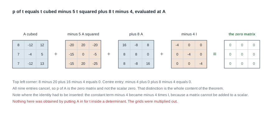
Take the top left corner: \(8 - 20 + 16 - 4 = 0\). The centre entry: \(-4 - 0 + 8 - 4 = 0\). Row two, column three: \(5 - 5 + 0 - 0 = 0\). All nine cancel, and the figure lays out the four grids so you can check any entry without re-multiplying. What this establishes is that \(p_A(A)\) is the zero matrix; what it does not establish is the theorem, since one example never does.
The same reasoning, transferred
Run the same opening steps — characteristic polynomial, candidate divisors, test the smallest — on a matrix where the two polynomials come apart, then put the shorter one to work. Over \(\mathbb{Q}\) take \[B = \begin{pmatrix} 3 & 1 & 1 \\ 1 & 3 & 1 \\ 1 & 1 & 3 \end{pmatrix} .\] Then \(\operatorname{tr} B = 9\), each principal \(2 \times 2\) minor is \(9 - 1 = 8\) so \(\sigma_2 = 24\), and \(\det B = 3(9-1) - 1(3-1) + 1(1-3) = 24 - 2 - 2 = 20\). So \(p_B(t) = t^3 - 9t^2 + 24t - 20 = (t-5)(t-2)^2\), the same shape as before. Test the smaller candidate: \(B - 5I\) has rows \((-2,1,1)\), \((1,-2,1)\), \((1,1,-2)\), while \(B - 2I\) is the all-ones matrix, every column \((1,1,1)\). Each row of \(B - 5I\) sums to zero, so \((B - 5I)(B - 2I) = 0\) and \(m_B(t) = (t-5)(t-2)\), a proper divisor of \(p_B\). Distinct linear factors, so \(B\) is diagonalizable — as Week 12 predicted independently, since \(B\) is real symmetric.
Now use \(m_B\) to invert. From \(B^2 - 7B + 10I = 0\) we get \(10I = 7B - B^2 = B(7I - B)\), so \[B^{-1} = \tfrac{1}{10}\,(7I - B) = \tfrac{1}{10} \begin{pmatrix} 4 & -1 & -1 \\ -1 & 4 & -1 \\ -1 & -1 & 4 \end{pmatrix} .\] Verify by multiplying: row one of \(B\) is \((3,1,1)\), and against the columns \((4,-1,-1)\), \((-1,4,-1)\), \((-1,-1,4)\) it gives \(12 - 1 - 1 = 10\), then \(-3 + 4 - 1 = 0\), then \(-3 - 1 + 4 = 0\). Rows two and three behave the same way by symmetry, so \(B(7I - B) = 10I\) and \(BB^{-1} = I\).
What stayed the same: the divisor test, the order of the candidates, and the shared roots of \(m\) and \(p\). What changed: the minimal polynomial is now a proper divisor, the operator is diagonalizable, and the inversion formula is quadratic rather than cubic. Running the same trick from \(p_B\) would give \(B^{-1} = \tfrac{1}{20}(B^2 - 9B + 24I)\) — the same matrix, since \(B^2 - 9B + 24I\) has diagonal \(8\) and off-diagonal \(-2\), exactly twice \(7I - B\) — at the cost of one more matrix product. The trick works exactly when the constant term of the annihilating polynomial is nonzero, that is, when \(0\) is not an eigenvalue.
Second worked example — one characteristic polynomial, two operators
This example shows that \(p_T\) alone does not determine an operator up to similarity, and locates how much it misses. Work over \(\mathbb{C}\) with \(V = \mathbb{C}^2\) and the two operators given in the standard basis by \[D = \begin{pmatrix} 2 & 0 \\ 0 & 2 \end{pmatrix}, \qquad J = \begin{pmatrix} 2 & 1 \\ 0 & 2 \end{pmatrix} .\] Both are upper triangular with diagonal \(2, 2\), so \(p_D(t) = p_J(t) = (t-2)^2\) by the diagonal reading above. Both are already in Schur form, with \(U = I\).
The minimal polynomials differ. \(D - 2I = 0\), so \(t - 2\) annihilates \(D\) and \(m_D(t) = t - 2\); no constant polynomial annihilates a nonzero operator, so this is minimal. For \(J\), \(J - 2I = \begin{pmatrix} 0 & 1 \\ 0 & 0 \end{pmatrix} \ne 0\), so \(t - 2\) fails, while \((J - 2I)^2 = 0\) by direct multiplication. Hence \(m_J(t) = (t-2)^2\). The test reports what we expect: \(m_D\) has a single linear factor and \(D\) is diagonal already, while \(m_J\) repeats and \(J\) is not diagonalizable.
They are not similar, and the proof is one line. If \(J = P^{-1}DP\) for some invertible \(P\), then since \(D = 2I\) commutes with everything, \(P^{-1}DP = 2P^{-1}P = 2I = D \ne J\). So no such \(P\) exists — and a scalar operator is therefore alone in its similarity class.
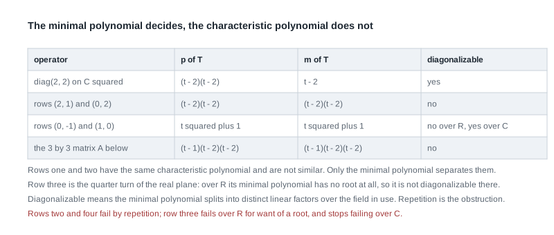
The table gathers the four examples this page has used. Rows one and two agree in the second column and disagree in the third and fourth, which is the whole point. Row three shows the other failure mode, where the minimal polynomial has no root in the field at all, repaired by enlarging the field. Row four is the worked example, where \(m\) and \(p\) coincide and the operator is defective anyway.
How far the minimal polynomial gets you, and no further. It is tempting to conclude that \(p_T\) and \(m_T\) together classify operators. They do not, and the smallest failure needs dimension four. Over \(\mathbb{C}\) let \(M_1\) be block diagonal built from two copies of \(\begin{pmatrix} 2 & 1 \\ 0 & 2 \end{pmatrix}\), and let \(M_2\) be built from one copy of that block together with two diagonal entries equal to \(2\). Both are \(4 \times 4\) upper triangular with every diagonal entry \(2\), so \(p(t) = (t-2)^4\) for each; and \((M_i - 2I)^2 = 0\) while \(M_i - 2I \ne 0\), so \(m(t) = (t-2)^2\) for each. Yet they are not similar: \(M_1 - 2I\) has rank \(2\) and \(M_2 - 2I\) has rank \(1\), and rank is a similarity invariant by Week 4. The missing datum is the rank sequence of the powers of \(T - \lambda I\), and supplying it is what Weeks 14 and 15 do.
The misreading to avoid
The misreading: Cayley-Hamilton is obvious — put \(A\) in for \(t\) in \(p_A(t) = \det(tI - A)\) and you get \(\det(A - A) = \det 0 = 0\), so \(p_A(A) = 0\). This is stated confidently every year and it is not a proof of anything.
Start with the type mismatch, which is fatal on its own. The function \(t \mapsto \det(tI - A)\) takes a scalar and returns a scalar. The expression \(\det(A \cdot I - A)\) takes a matrix and returns a scalar, namely the number \(0\). But Cayley-Hamilton asserts that \(p_A(A)\) is the zero matrix, an \(n \times n\) array. A derivation whose output is a number cannot establish a statement about an array; the two zeros live in different spaces. In the figure of the collapsing grids, what was verified was nine entries vanishing, not one determinant vanishing.
Now the deeper error, which survives even if you wave at the mismatch. Evaluating a polynomial at a matrix requires the polynomial as a formal expression in \(t\) first. Here \(p_A(t) = t^3 - 5t^2 + 8t - 4\), and by definition \(p_A(A) = A^3 - 5A^2 + 8A - 4I\). Look at the last term: the constant \(-4\) became \(-4I\). That insertion of the identity is part of the definition of evaluation at an operator and has no counterpart inside the determinant expression. The bogus argument never produces the term \(-4I\) at all, so whatever it computes, it is not \(p_A(A)\).
A third angle finishes it. If substituting a matrix into a determinant were legal it would be legal in general, and it is not: \(tI - A\) has entries that are polynomials in \(t\), so replacing \(t\) by an \(n \times n\) matrix turns each entry into an \(n \times n\) block and the object under the determinant becomes \(n^2 \times n^2\). A genuine theorem does hide in that direction — work in the ring of matrices with polynomial entries and use the adjugate identity \(\operatorname{adj}(tI - A)\,(tI - A) = p_A(t)I\) — but the honest version needs care about which ring each symbol lives in. The Schur argument above sidesteps the issue by never substituting anything.
One related habit to correct. Cayley-Hamilton does not say \(p_T\) is the smallest relation an operator satisfies. It says \(p_T\) is one relation; the smallest is \(m_T\), often strictly smaller, as \(B\) showed with \(\deg m_B = 2 < 3 = \deg p_B\). Reaching for \(p_T\) when you meant \(m_T\) costs extra powers in every computation and hides the diagonalizability test, since a repeated root of \(p_T\) says nothing about whether \(T\) is diagonalizable.
Practice on your own
These are for your own checking rather than for submission, and each is within reach of Weeks 10 through 13.
- A Schur form by hand. Let \(A = \begin{pmatrix} 3 & 1 \\ -1 & 1 \end{pmatrix}\) over \(\mathbb{C}\). Show \(p_A(t) = (t-2)^2\), find a unit eigenvector, extend it to an orthonormal basis, and compute \(U^{*}AU\). Confirm it is upper triangular with \(2\) on the diagonal, then say why no \(U\) makes it diagonal.
- Minimal polynomial of differentiation. Let \(D\) be differentiation on \(P_3(\mathbb{R})\), of dimension four. Compute \(p_D\) and \(m_D\), and decide diagonalizability. Then redo it on \(P_3(\mathbb{F}_2)\), where \(D(x^2) = 2x = 0\), and explain why \(m_D\) drops in degree while \(p_D\) does not.
- Where a hypothesis is doing work. In the proof of Schur’s theorem, identify the step that uses algebraic closure of \(\mathbb{C}\) and the step that uses finite-dimensionality. Then show by example that the theorem fails over \(\mathbb{R}\), and state a hypothesis on \(A\) that repairs it.
- Inverses from annihilating polynomials. Let \(C = \begin{pmatrix} 1 & 2 \\ 3 & 4 \end{pmatrix}\) over \(\mathbb{Q}\). Compute \(p_C\), use Cayley-Hamilton to write \(C^{-1}\) as a polynomial in \(C\), and check the product. Then say why the route fails precisely when \(\det C = 0\), arguing from the constant term of \(p_C\).
- Reconstructing an operator from its relations. Suppose \(T\) on a five-dimensional complex space satisfies \((T - 3I)^2(T - 7I) = 0\) but neither \((T-3I)(T-7I) = 0\) nor \((T-3I)^2 = 0\). Determine \(m_T\), list the possibilities for \(p_T\), and say what you can and cannot conclude about \(\operatorname{geo}(3)\).
Where to read more
This page stands on its own, but a second treatment in a different voice is often what makes a theorem settle. The three addresses below are offered online at no cost by their providers; availability and licence terms are as those providers state them, and neither is confirmed here.
- MIT OpenCourseWare 18.700 Linear Algebra — a proof-based course whose treatment of triangular forms, annihilating polynomials, and Cayley-Hamilton runs parallel to this week.
- Linear Algebra Done Wrong by Sergei Treil — an abstract-first text whose chapter on the structure of operators develops the Schur form and the polynomial machinery in the order used here.
- MIT OpenCourseWare 18.06 Linear Algebra — the computational complement, for exercising characteristic polynomials and powers of matrices on explicit numerical arrays.
- The optional Roman alignment for this week is the chapter on eigenvalues and eigenvectors, in the sections on triangularization, on the minimal polynomial, and on the Cayley-Hamilton theorem. That text is an optional reference: a borrowed or library copy suffices, and nothing from it is reproduced here.
- Course pages: the notes overview, the syllabus, the schedule, and the resources page. The learning management system remains authoritative for section logistics and graded details.
Where this goes next
You now hold two tools that survive the failure of diagonalizability. Schur’s theorem gives every complex operator a triangular matrix in an orthonormal basis, so the eigenvalues are visible and the obstruction is confined above the diagonal. The minimal polynomial gives the exact relation an operator satisfies, divides \(p_T\) by Cayley-Hamilton, shares its roots, and decides diagonalizability by whether its linear factors repeat. What neither tool does is classify: the \(4 \times 4\) pair above agreed on both polynomials and were still not similar.
Week 14, on generalized eigenvectors, nilpotent operators, and primary decomposition, attacks that gap from the side the star entries point to. Instead of \(E_{\lambda} = \ker(T - \lambda I)\), too small when \(\operatorname{geo}(\lambda) < \operatorname{alg}(\lambda)\), it uses the generalized eigenspace \(G_{\lambda} = \ker\big((T - \lambda I)^{\dim V}\big)\), shows those do fill the space when \(p_T\) splits, and isolates the one hard case: an operator whose only eigenvalue is zero. Week 15 then assembles the Jordan canonical form and closes the similarity question Week 4 opened. To look back instead: Week 12 carries the spectral theorem this page rederived from Schur, and the notes index and course home page list what is here.