Week 11 — Similar matrices, diagonalization, and multiplicity

Where this week starts

Week 4 left a promissory note. It showed that changing the ordered basis of one space moves the matrix of an operator by \(A \mapsto PAP^{-1}\), named that relation similarity, proved that rank settles matrix equivalence completely, and then admitted that rank settles similarity not at all. Week 10 collected the tools to do better: eigenvalues, eigenvectors, the characteristic polynomial \(p_T(t) = \det(tI - T)\) in that sign convention, eigenspaces, and the fact that an operator on a nonzero finite-dimensional complex space always has an eigenvalue while the quarter-turn rotation of \(\mathbb{R}^2\) has none.

This week spends those tools on the first serious question about a similarity class: does it contain a diagonal matrix? Such an array carries \(n\) numbers instead of \(n^2\), its powers are computed entrywise, and every question about it splits into \(n\) independent one-dimensional questions. If the class contains one, the operator is understood; if not, you want to know what obstructed it.

The obstruction is a comparison of two numbers attached to each eigenvalue. The algebraic multiplicity counts how many times \(\lambda\) occurs as a root of \(p_T\); the geometric multiplicity counts how many independent eigenvectors \(\lambda\) actually supplies. The first is always at least the second, and equality at every eigenvalue — together with \(p_T\) splitting over the field you are working in — is exactly the condition for diagonalizability.

Three habits should be automatic by the end. Ask what a similarity class remembers. At a repeated eigenvalue, neither panic nor relax: compute \(\dim \ker(T - \lambda I)\) and compare. And when someone says “diagonalizable”, ask over which field, because one array of integers can be diagonalizable over \(\mathbb{C}\) and not over \(\mathbb{R}\).

Why this matters beyond the definition

Here is a concrete failure this material prevents. Somebody wants \(A^{20}\) for the \(3 \times 3\) matrix below and multiplies \(A\) by itself nineteen times, thousands of scalar products and one slip away from being wrong. Diagonalising costs one characteristic polynomial, three small null spaces, and one inversion, after which \(A^{20} = PD^{20}P^{-1}\) and \(D^{20}\) is three numbers on a diagonal. The arithmetic saving is secondary; the structure is the gain. Once you see \(A^{k} = PD^{k}P^{-1}\), every entry of \(A^{k}\) is visibly a fixed combination of \(1^{k}\), \(2^{k}\), \(3^{k}\) — which is why linear recurrences have the closed forms they do.

The second stake is a wrong proof rather than a wrong number. A student wants two matrices to be similar, checks that their characteristic polynomials agree, and declares it done. That inference is invalid, and the smallest counterexample is \(2I_2\) against the array with \(2\) on the diagonal and a single \(1\) above it: same characteristic polynomial \((t-2)^2\), same trace, determinant, and rank. They are not similar, because \(P^{-1}(2I_2)P = 2I_2\) for every invertible \(P\). The invariant list is real and it is incomplete, and knowing which is which separates a proof from a guess.

What you will be able to do

• State what it means for two matrices over \(F\) to be similar, and prove that trace, determinant, rank, characteristic polynomial, and both multiplicities of every eigenvalue are similarity invariants.
• Prove by induction that eigenvectors belonging to distinct eigenvalues are independent, without assuming \(V\) is finite-dimensional.
• Prove that an operator on a finite-dimensional space is diagonalizable exactly when the space has a basis of eigenvectors, and locate that basis inside \(P\).
• Prove \(1 \le \operatorname{geo}(\lambda) \le \operatorname{alg}(\lambda)\), naming where finite-dimensionality enters.
• Decide diagonalizability over a named field, and exhibit an operator diagonalizable over \(\mathbb{C}\) and not over \(\mathbb{R}\).
• Diagonalise an explicit matrix, verify \(P^{-1}AP = D\) by multiplying out, and use it to compute a high power.

Terms and notation worth fixing

Symbol or term	What it means on this page
\(A \sim B\)	similar over \(F\): \(B = P^{-1}AP\) for some invertible \(P\) with entries in \(F\)
\(p_T(t) = \det(tI - T)\)	the characteristic polynomial, monic of degree \(\dim V\), always in this sign convention
\(E_{\lambda} = \ker(T - \lambda I)\)	the eigenspace of \(\lambda\): every eigenvector for \(\lambda\), together with \(0\)
\(\operatorname{alg}(\lambda)\)	algebraic multiplicity: how many times \(t - \lambda\) divides \(p_T(t)\)
\(\operatorname{geo}(\lambda)\)	geometric multiplicity: \(\dim E_{\lambda}\), the count of independent eigenvectors for \(\lambda\)
\(p_T\) splits over \(F\)	\(p_T(t) = (t - \lambda_1)^{a_1} \cdots (t - \lambda_k)^{a_k}\) with every \(\lambda_i \in F\)
diagonalizable over \(F\)	similar over \(F\) to some \(D = \operatorname{diag}(d_1, \dots, d_n)\)
defective	some eigenvalue has \(\operatorname{geo}(\lambda) < \operatorname{alg}(\lambda)\), so no eigenbasis exists

Similarity, and the invariants it cannot move

Two square matrices over \(F\) are similar when one is \(P^{-1}AP\) for an invertible \(P\) over \(F\). Week 4 derived that relation rather than declaring it: it is what the change-of-basis law becomes when one space sits at both ends of the map, as it must whenever the map is an operator you intend to compose with itself.

Similarity is one change of basis, seen twice

Let \(V\) be finite-dimensional over \(F\) with \(\dim V = n\), let \(T \in \mathcal{L}(V)\), and let \(\mathcal{B}\), \(\mathcal{C}\) be ordered bases of \(V\). Write \(A = [T]_{\mathcal{B} \leftarrow \mathcal{B}}\) and \(B = [T]_{\mathcal{C} \leftarrow \mathcal{C}}\), reading the subscripts right to left as Week 4 fixed them. With \(P = P_{\mathcal{B} \leftarrow \mathcal{C}}\), whose \(j\)-th column is the \(\mathcal{B}\)-coordinate column of the \(j\)-th member of \(\mathcal{C}\), \[B = P_{\mathcal{C} \leftarrow \mathcal{B}}\,[T]_{\mathcal{B} \leftarrow \mathcal{B}}\,P_{\mathcal{B} \leftarrow \mathcal{C}} = P^{-1}AP .\] Conversely, any invertible \(P\) over \(F\) is the change-of-basis matrix of exactly one ordered basis, the one whose members have the columns of \(P\) as \(\mathcal{B}\)-coordinates: those columns are independent because \(P\) is invertible, and \(n\) independent vectors in an \(n\)-dimensional space form a basis by Week 2. So similar matrices and two records of one operator say the same thing. Similarity is an equivalence relation on \(M_n(F)\): reflexive with \(P = I_n\), symmetric via \(P^{-1}\), transitive because \((PQ)^{-1}A(PQ) = Q^{-1}(P^{-1}AP)Q\).

The field is part of the statement, since \(P\) must have entries in \(F\). Enlarging the field can only make more pairs similar: the rotation matrix \(R = \begin{pmatrix} 0 & -1 \\ 1 & 0 \end{pmatrix}\) is similar over \(\mathbb{C}\) to \(\operatorname{diag}(i, -i)\) and over \(\mathbb{R}\) to no diagonal matrix at all.

Trace, determinant, rank, and the characteristic polynomial

A similarity invariant is a quantity computed from a matrix that agrees on similar matrices. Each proof below is short enough to reproduce from memory.

Proposition (trace). For \(A, B \in M_n(F)\), \(\operatorname{tr}(AB) = \operatorname{tr}(BA)\); hence \(\operatorname{tr}(P^{-1}AP) = \operatorname{tr}(A)\) for every invertible \(P\).

Argument. By definition \(\operatorname{tr}(AB) = \sum_{i} (AB)_{ii} = \sum_{i} \sum_{j} A_{ij}B_{ji}\). That double sum is finite, so grouping by \(j\) first gives \(\sum_{j} \sum_{i} B_{ji}A_{ij} = \operatorname{tr}(BA)\); only commutativity of multiplication in \(F\) was used. Applying it to \(X = P^{-1}A\) and \(Y = P\) gives \(\operatorname{tr}(P^{-1}AP) = \operatorname{tr}(PP^{-1}A) = \operatorname{tr}(A)\).

Proposition. Each of \(\det A\), \(\operatorname{rank} A\), and \(p_A(t) = \det(tI - A)\) agrees on similar matrices.

Argument. Multiplicativity of the determinant — a MATH 3312 fact this course uses rather than rebuilds — gives \(\det(P^{-1}AP) = \det(P)^{-1}\det(A)\det(P) = \det A\), legitimate because \(\det P\) is a nonzero element of the field \(F\). Week 4 showed that multiplying on either side by an invertible matrix leaves rank unchanged, since invertible matrices represent isomorphisms and an isomorphism changes no image dimension. For the polynomial, \(tI - P^{-1}AP = P^{-1}(tI - A)P\), because \(P^{-1}(tI)P = tI\); taking determinants and reusing the first computation gives \(p_{P^{-1}AP} = p_A\).

Corollary. If \(A \sim B\) then they share their eigenvalues, and for each \(\lambda\) both multiplicities.

Argument. Eigenvalues are the roots of the shared polynomial in \(F\), with algebraic multiplicities their root multiplicities. And \(B - \lambda I = P^{-1}(A - \lambda I)P\) has the rank of \(A - \lambda I\), so rank-nullity in the fixed dimension \(n\) turns equal ranks into equal nullities, which are the two geometric multiplicities.

One consequence ties the list together. If \(p_A\) splits over \(F\) as \(\prod_{i=1}^{n}(t - \mu_i)\) with repetitions listed, comparing the coefficient of \(t^{n-1}\) and the constant term against the determinant expansion gives \(\sum_i \mu_i = \operatorname{tr} A\) and \(\prod_i \mu_i = \det A\). So once \(p_A\) splits, trace and determinant are two of its coefficients and carry nothing beyond it — but they stay the cheapest check on a computation, and the worked example uses them that way twice.

What the invariant list still fails to settle

What each similarity invariant is, and the pair it cannot separate.

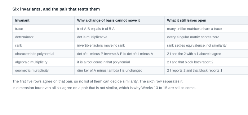
Read the table’s right-hand column downward and the shape of the week appears. The first five rows agree on the pair \(2I_2\) and \(\begin{pmatrix} 2 & 1 \\ 0 & 2 \end{pmatrix}\): characteristic polynomial \((t-2)^2\), trace \(4\), determinant \(4\), rank \(2\), \(\operatorname{alg}(2) = 2\). Only the last row separates them, with \(\operatorname{geo}(2)\) equal to \(2\) on the left and \(1\) on the right.

Even the full list is incomplete, better learned now than in Week 15. In dimension four over any field, compare the matrix built from two blocks of size two with \(0\) on the diagonal and \(1\) above it against the one built from a block of size three and a block of size one, both with \(0\) on the diagonal. Each has characteristic polynomial \(t^4\), so \(\operatorname{alg}(0) = 4\); each has rank \(2\), so \(\operatorname{geo}(0) = 2\). Yet the first squares to zero and the second does not, and \((P^{-1}AP)^2 = P^{-1}A^2P\) vanishes exactly when \(A^2\) does, so they are not similar. Deciding similarity in general needs Week 13’s minimal polynomial and Week 15’s block structure; this week settles the one case where that machinery collapses to nothing.

Diagonalizability and the two multiplicities

Fix \(V\) finite-dimensional over \(F\) with \(\dim V = n \ge 1\) and \(T \in \mathcal{L}(V)\). Call \(T\) diagonalizable over \(F\) when some ordered basis \(\mathcal{C}\) makes \([T]_{\mathcal{C} \leftarrow \mathcal{C}}\) diagonal. This section unpacks that definition into something you can check.

Eigenvectors for distinct eigenvalues are independent

Theorem. Let \(V\) be a vector space over \(F\), let \(T \in \mathcal{L}(V)\), let \(\lambda_1, \dots, \lambda_m\) be pairwise distinct eigenvalues of \(T\), and let \(v_i\) be an eigenvector for \(\lambda_i\). Then \(v_1, \dots, v_m\) are linearly independent.

Argument, by induction on \(m\). For \(m = 1\): an eigenvector is nonzero by definition, and \(a v_1 = 0\) with \(a \ne 0\) would give \(v_1 = a^{-1}(av_1) = 0\), which is where \(F\) being a field rather than a ring is used. Assume the statement for \(m - 1\) and let \(a_1 v_1 + \dots + a_m v_m = 0\). Apply \(T - \lambda_m I\) to both sides: the \(i\)-th term becomes \(a_i(\lambda_i - \lambda_m)v_i\) and the \(m\)-th vanishes, so \[a_1(\lambda_1 - \lambda_m)v_1 + \dots + a_{m-1}(\lambda_{m-1} - \lambda_m)v_{m-1} = 0 .\] The eigenvalues \(\lambda_1, \dots, \lambda_{m-1}\) are still pairwise distinct, so the inductive hypothesis kills every coefficient: \(a_i(\lambda_i - \lambda_m) = 0\) for \(i < m\). Each \(\lambda_i - \lambda_m\) is a nonzero element of \(F\), hence invertible, so \(a_i = 0\) there. What remains is \(a_m v_m = 0\) with \(v_m \ne 0\), forcing \(a_m = 0\).

Notice what the proof never assumed. It did not mention \(\dim V\), so it holds verbatim in infinite-dimensional spaces such as \(F^{\mathbb{N}}\); it did not require \(F\) algebraically closed; it touched no basis and no matrix. What it used is distinctness, in the step inverting \(\lambda_i - \lambda_m\).

Corollary. If \(\dim V = n\) is finite, \(T\) has at most \(n\) distinct eigenvalues; and if it has exactly \(n\) of them in \(F\), one eigenvector for each gives a basis of \(V\), so \(T\) is diagonalizable over \(F\).

Argument. Week 2 caps an independent set in an \(n\)-dimensional space at \(n\) members, and \(n\) independent vectors there form a basis. The next subsection turns a basis of eigenvectors into a diagonal matrix.

An eigenbasis, and where it sits in P

Theorem. Let \(\dim V = n\) be finite. Then \(T\) is diagonalizable over \(F\) if and only if \(V\) has a basis of eigenvectors of \(T\). In matrix terms, for \(A \in M_n(F)\) the equation \(P^{-1}AP = \operatorname{diag}(d_1, \dots, d_n)\) holds for an invertible \(P\) exactly when the columns \(p_1, \dots, p_n\) of \(P\) form a basis of \(F^n\) with \(Ap_j = d_j p_j\) for every \(j\).

Argument. Suppose \(\mathcal{C} = (u_1, \dots, u_n)\) is a basis with \([T]_{\mathcal{C} \leftarrow \mathcal{C}} = D\) diagonal. Its \(j\)-th column is \([Tu_j]_{\mathcal{C}}\) by the column-by-column definition, and being diagonal that column holds \(d_j\) in slot \(j\) and zeros elsewhere, which says \(Tu_j = d_j u_j\); each \(u_j\) is a basis vector, hence nonzero, hence an eigenvector. Run the computation backwards for the converse. For the matrix form, \(P^{-1}AP = D\) is equivalent to \(AP = PD\); the \(j\)-th column of \(AP\) is \(Ap_j\) and the \(j\)-th column of \(PD\) is \(d_j p_j\), so the equation says exactly \(Ap_j = d_j p_j\), while invertibility of \(P\) says exactly that its columns are a basis of \(F^n\).

Multiplying by A is: translate into eigen coordinates, scale, translate back.

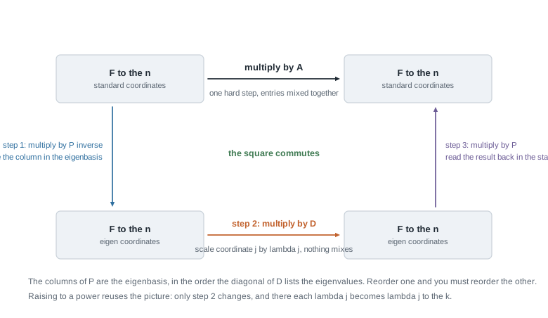
The square holds all of \(A = PDP^{-1}\), and it reads better as a route than as a formula. Right along the top is one hard step in which entries mix; down, right, and up is three easy ones: rewrite the column in the eigenbasis, scale coordinate \(j\) by \(\lambda_j\) so nothing mixes, then rewrite the result in the standard basis. Two consequences follow by inspection. The order of the columns of \(P\) must match the order of the diagonal entries of \(D\), since column \(j\) and slot \(j\) meet in \(Ap_j = d_jp_j\); and raising to a power changes only the bottom arrow, because \(A^k = PD^kP^{-1}\) once the interior cancellations \(P^{-1}P = I\) are performed.

Why geometric multiplicity never exceeds algebraic

Theorem. Let \(\dim V = n\) be finite and let \(\lambda \in F\) be an eigenvalue of \(T \in \mathcal{L}(V)\). Then \(1 \le \operatorname{geo}(\lambda) \le \operatorname{alg}(\lambda)\).

Argument. The lower bound is the definition: \(\lambda\) being an eigenvalue means \(T - \lambda I\) has nontrivial kernel. For the upper bound put \(g = \operatorname{geo}(\lambda)\), take a basis \((u_1, \dots, u_g)\) of \(E_{\lambda}\), and extend it to an ordered basis \(\mathcal{C}\) of \(V\) by Week 2’s extension theorem — the one place finite-dimensionality is genuinely needed, since without it no such extension is available by elementary means. For \(j \le g\) we have \(Tu_j = \lambda u_j\), so the first \(g\) columns of \(M = [T]_{\mathcal{C} \leftarrow \mathcal{C}}\) are \(\lambda\) times the first \(g\) standard columns, giving the block form \[M = \begin{pmatrix} \lambda I_g & B \\ 0 & C \end{pmatrix}, \qquad tI_n - M = \begin{pmatrix} (t - \lambda)I_g & -B \\ 0 & tI_{n-g} - C \end{pmatrix}\] with \(C\) of size \((n-g) \times (n-g)\). The determinant of a block upper triangular matrix is the product of the determinants of its diagonal blocks — again MATH 3312 determinant theory, used and not rebuilt — so \(p_T(t) = (t - \lambda)^{g}\det(tI_{n-g} - C)\), this being the characteristic polynomial itself because \(p_T\) is a similarity invariant and may be computed in any basis. Hence \((t-\lambda)^g\) divides \(p_T\), which says \(\operatorname{alg}(\lambda) \ge g\).

Nothing forbids the leftover factor \(\det(tI_{n-g} - C)\) from carrying further copies of \(t - \lambda\), and that is precisely how the inequality becomes strict.

The criterion, and the easy sufficient condition

Lemma (eigenspaces are independent). Let \(\lambda_1, \dots, \lambda_k\) be the distinct eigenvalues of \(T\) in \(F\). If \(u_1 + \dots + u_k = 0\) with \(u_i \in E_{\lambda_i}\), then every \(u_i = 0\); consequently the sum \(E_{\lambda_1} + \dots + E_{\lambda_k}\) is direct, and concatenating a basis of each eigenspace gives an independent list.

Argument. Discard the indices with \(u_i = 0\). Any survivors would be eigenvectors for pairwise distinct eigenvalues summing to zero with all coefficients \(1\), contradicting the theorem above, so none survive. For the second claim, suppose a combination of the concatenated bases vanishes: group the terms by eigenspace, let \(u_i\) be the \(i\)-th group’s sum, apply the first claim, and then independence inside \(E_{\lambda_i}\) kills that group’s coefficients. Directness is Week 1’s characterisation by uniqueness of the zero expression.

Theorem (the diagonalizability criterion). Let \(V\) be finite-dimensional over \(F\) with \(\dim V = n \ge 1\) and let \(T \in \mathcal{L}(V)\) have distinct eigenvalues \(\lambda_1, \dots, \lambda_k\) in \(F\). Then \(T\) is diagonalizable over \(F\) if and only if \(p_T\) splits into linear factors over \(F\) and \(\operatorname{geo}(\lambda_i) = \operatorname{alg}(\lambda_i)\) for every \(i\).

Argument. Suppose both hold. A monic polynomial of degree \(n\) that splits is a product of exactly \(n\) linear factors, so \(\sum_i \operatorname{alg}(\lambda_i) = n\), and matching multiplicities turns that into \(\sum_i \dim E_{\lambda_i} = n\). The lemma makes the concatenated eigenspace bases independent, and an independent list of \(n\) members in an \(n\)-dimensional space is a basis by Week 2 — a basis of eigenvectors, hence diagonalizability. Conversely let \([T]_{\mathcal{C} \leftarrow \mathcal{C}} = D\) be diagonal with entries \(d_1, \dots, d_n\). Then \(p_T(t) = \prod_{j}(t - d_j)\) splits over \(F\), and \(\operatorname{alg}(\lambda_i)\) is the number \(a_i\) of times \(\lambda_i\) appears on the diagonal. Those \(a_i\) members of \(\mathcal{C}\) are independent vectors inside \(E_{\lambda_i}\), so \(\operatorname{geo}(\lambda_i) \ge a_i\), and the previous theorem gives equality.

Two special cases travel separately. First, \(n\) distinct eigenvalues in \(F\) force every \(\operatorname{alg}\) to be \(1\), and \(1 \le \operatorname{geo} \le \operatorname{alg} = 1\) leaves no room, so the corollary above is the degenerate case of the criterion — sufficient, and emphatically not necessary, since \(I_n\) has one eigenvalue and is already diagonal. Second, splitting is not automatic: free over \(\mathbb{C}\) by the fundamental theorem of algebra used in Week 10, a real condition over \(\mathbb{R}\) that the quarter-turn rotation with \(p_R(t) = t^2 + 1\) fails, and failed over \(\mathbb{Q}\) even by \(\begin{pmatrix} 0 & 2 \\ 1 & 0 \end{pmatrix}\), whose \(p(t) = t^2 - 2\) is irreducible there and splits over \(\mathbb{R}\).

Commuting operators, diagonalised together

Theorem (simultaneous diagonalization). Let \(V\) be finite-dimensional over \(F\) and let \(S, T \in \mathcal{L}(V)\) both be diagonalizable over \(F\). If \(ST = TS\), then \(V\) has a basis of vectors that are eigenvectors of \(S\) and of \(T\) at once, so one invertible \(P\) makes both matrices diagonal. Conversely, simultaneously diagonalizable operators commute.

Sketch, with the compressed step named. The converse is immediate: diagonal matrices commute entrywise, so \(P^{-1}AP = D_1\) and \(P^{-1}BP = D_2\) give \(AB = PD_1D_2P^{-1} = BA\). Forwards, each eigenspace of \(T\) is invariant under \(S\), since \(Tv = \lambda v\) gives \(T(Sv) = S(Tv) = \lambda(Sv)\), and diagonalizability of \(T\) gives \(V = E_{\lambda_1} \oplus \dots \oplus E_{\lambda_k}\). The step being compressed: the restriction of a diagonalizable operator to an invariant subspace is again diagonalizable. Granting it, choose in each \(E_{\lambda_i}\) a basis of eigenvectors of \(S|_{E_{\lambda_i}}\); every such vector is an eigenvector of \(S\) and, lying in \(E_{\lambda_i}\), of \(T\) as well, so concatenating over \(i\) gives the basis claimed. Week 13 proves the compressed step from the minimal polynomial of a restriction dividing that of the whole operator. The diagonalizability hypothesis matters: \(\begin{pmatrix} 0 & 1 \\ 0 & 0 \end{pmatrix}\) commutes with itself and is diagonalizable over no field, so commuting alone buys nothing. The commuting hypothesis matters too, and the fifth practice item below asks you to build the pair that shows it.

Worked example — diagonalising a three-by-three matrix and taking its fifth power

Work over \(\mathbb{R}\) with \(V = \mathbb{R}^3\), and let \(T\) have matrix \[A = \begin{pmatrix} 0 & 0 & 1 \\ -2 & 1 & 2 \\ -2 & -2 & 5 \end{pmatrix}\] in the standard basis. Find the eigenvalues and an eigenbasis, assemble \(P\) and \(P^{-1}\), verify \(P^{-1}AP = D\) by multiplying out, then compute \(A^5\) two independent ways.

Step 1. The characteristic polynomial. Expand \(\det(tI - A)\) along the first row: \[tI - A = \begin{pmatrix} t & 0 & -1 \\ 2 & t-1 & -2 \\ 2 & 2 & t-5 \end{pmatrix},\] \[p_A(t) = t\big[(t-1)(t-5) + 4\big] - \big[2 \cdot 2 - 2(t-1)\big] = t(t^2 - 6t + 9) - (6 - 2t) = t^3 - 6t^2 + 11t - 6 .\] Two checks before factoring: the coefficient of \(t^2\) should be \(-\operatorname{tr} A = -6\), and it is; the constant term should be \(-\det A\), and expanding \(\det A\) along its first row gives \(1 \cdot \big[(-2)(-2) - (1)(-2)\big] = 6\). Since \(p_A(1) = 1 - 6 + 11 - 6 = 0\), dividing by \(t - 1\) leaves \(t^2 - 5t + 6\), so \[p_A(t) = (t-1)(t-2)(t-3) .\] Three distinct eigenvalues in \(\mathbb{R}\), each with \(\operatorname{alg} = 1\), so the corollary already grants diagonalizability; the eigenvectors are still needed to build \(P\).

Step 2. The eigenspaces. For \(\lambda = 1\), \(A - I = \begin{pmatrix} -1 & 0 & 1 \\ -2 & 0 & 2 \\ -2 & -2 & 4 \end{pmatrix}\): row one gives \(z = x\), and row three then gives \(2x - 2y = 0\), so \(y = x\) and \(E_1 = \operatorname{span}\{(1,1,1)\}\). For \(\lambda = 2\), \(A - 2I = \begin{pmatrix} -2 & 0 & 1 \\ -2 & -1 & 2 \\ -2 & -2 & 3 \end{pmatrix}\): row one gives \(z = 2x\), row two then gives \(2x - y = 0\), so \(E_2 = \operatorname{span}\{(1,2,2)\}\). For \(\lambda = 3\), \(A - 3I = \begin{pmatrix} -3 & 0 & 1 \\ -2 & -2 & 2 \\ -2 & -2 & 2 \end{pmatrix}\): row one gives \(z = 3x\), row two then gives \(4x - 2y = 0\), so \(E_3 = \operatorname{span}\{(1,2,3)\}\). Each geometric multiplicity is \(1\), and each vector checks directly: \(A(1,1,1)^{\mathsf{T}} = (1,\,-2+1+2,\,-2-2+5)^{\mathsf{T}} = (1,1,1)^{\mathsf{T}}\); \(A(1,2,2)^{\mathsf{T}} = (2,\,-2+2+4,\,-2-4+10)^{\mathsf{T}} = 2(1,2,2)^{\mathsf{T}}\); \(A(1,2,3)^{\mathsf{T}} = (3,\,-2+2+6,\,-2-4+15)^{\mathsf{T}} = 3(1,2,3)^{\mathsf{T}}\).

Step 3. \(P\) and \(P^{-1}\). Put the eigenvectors in as columns in the order \(1, 2, 3\): \[P = \begin{pmatrix} 1 & 1 & 1 \\ 1 & 2 & 2 \\ 1 & 2 & 3 \end{pmatrix}, \quad \det P = 1(6-4) - 1(3-2) + 1(2-2) = 1, \quad P^{-1} = \begin{pmatrix} 2 & -1 & 0 \\ -1 & 2 & -1 \\ 0 & -1 & 1 \end{pmatrix} .\] Determinant \(1\) is why the inverse has integer entries. Check \(P^{-1}P\): row \((2,-1,0)\) against the columns of \(P\) gives \(1, 0, 0\); row \((-1,2,-1)\) gives \(0\), \(-1+4-2 = 1\), \(-1+4-3 = 0\); row \((0,-1,1)\) gives \(0\), \(0\), \(-2+3 = 1\).

Step 4. Verify \(P^{-1}AP = D\). The columns of \(AP\) are \(A\) applied to the columns of \(P\), computed in Step 2: \[AP = \begin{pmatrix} 1 & 2 & 3 \\ 1 & 4 & 6 \\ 1 & 4 & 9 \end{pmatrix} .\] Now \(P^{-1}(AP)\) row by row. Row \((2,-1,0)\) against the columns \((1,1,1)\), \((2,4,4)\), \((3,6,9)\) gives \(2-1 = 1\), \(4-4 = 0\), \(6-6 = 0\). Row \((-1,2,-1)\) gives \(-1+2-1 = 0\), \(-2+8-4 = 2\), \(-3+12-9 = 0\). Row \((0,-1,1)\) gives \(0\), \(-4+4 = 0\), \(-6+9 = 3\). So \(P^{-1}AP = \operatorname{diag}(1,2,3) = D\), every entry checkable with a pencil.

Step 5. The fifth power, structurally. Repeated multiplication cancels interior factors, so \(A^5 = PD^5P^{-1}\) with \(D^5 = \operatorname{diag}(1, 32, 243)\). Scaling the columns of \(P\) by those numbers and multiplying by \(P^{-1}\), \[PD^5 = \begin{pmatrix} 1 & 32 & 243 \\ 1 & 64 & 486 \\ 1 & 64 & 729 \end{pmatrix}, \qquad A^5 = \begin{pmatrix} -30 & -180 & 211 \\ -62 & -359 & 422 \\ -62 & -602 & 665 \end{pmatrix} .\] The first row is \((1, 32, 243)\) against the columns of \(P^{-1}\): \(2 - 32 = -30\), then \(-1 + 64 - 243 = -180\), then \(-32 + 243 = 211\). The other rows repeat those products with \((1,64,486)\) and \((1,64,729)\).

Step 6. Confirm it without the diagonalization. First, \(\operatorname{tr} A^5 = -30 - 359 + 665 = 276 = 1 + 32 + 243\), the sum of the fifth powers of the eigenvalues. Second, square by hand: \(A^2 = \begin{pmatrix} -2 & -2 & 5 \\ -6 & -3 & 10 \\ -6 & -12 & 19 \end{pmatrix}\) and \(A^4 = \begin{pmatrix} -14 & -50 & 65 \\ -30 & -99 & 130 \\ -30 & -180 & 211 \end{pmatrix}\). The first row of \(A\) is \((0,0,1)\), so the first row of \(A^5 = A \cdot A^4\) is the third row of \(A^4\), namely \((-30, -180, 211)\) — exactly Step 5. Every row of every power here sums to \(1\), which is \(A^k(1,1,1)^{\mathsf{T}} = (1,1,1)^{\mathsf{T}}\) for the eigenvalue \(1\).

So \(A\) is similar over \(\mathbb{R}\) to \(\operatorname{diag}(1,2,3)\), and its powers come in closed form: \(PD^kP^{-1}\) gives \((A^k)_{11} = 2 - 2^k\) and \((A^k)_{13} = 3^k - 2^k\), each entry a fixed integer combination of \(1^k\), \(2^k\), \(3^k\). It establishes nothing about a different matrix with the same characteristic polynomial, and it does not depend on \(\mathbb{R}\): every entry of \(A\), \(P\), \(P^{-1}\), \(D\) is an integer, so the identities hold over \(\mathbb{Q}\), \(\mathbb{C}\), and \(\mathbb{F}_5\). Over \(\mathbb{F}_2\), though, \(3 = 1\) and the eigenvalues collapse to two, so the argument reruns from Step 1.

The same reasoning, transferred

The same steps on a \(2 \times 2\) matrix fit in a paragraph. Let \(B = \begin{pmatrix} -1 & 3 \\ -6 & 8 \end{pmatrix}\) over \(\mathbb{R}\), so \(p_B(t) = t^2 - 7t + 10 = (t-2)(t-5)\), checked against \(\operatorname{tr} B = 7\) and \(\det B = -8 + 18 = 10\). For \(\lambda = 2\), \(B - 2I = \begin{pmatrix} -3 & 3 \\ -6 & 6 \end{pmatrix}\) has rank one and gives \(x = y\), so \((1,1)\); for \(\lambda = 5\), \(B - 5I = \begin{pmatrix} -6 & 3 \\ -6 & 3 \end{pmatrix}\) gives \(y = 2x\), so \((1,2)\). Then \(P = \begin{pmatrix} 1 & 1 \\ 1 & 2 \end{pmatrix}\) has \(\det P = 1\) and \(P^{-1} = \begin{pmatrix} 2 & -1 \\ -1 & 1 \end{pmatrix}\), and \(BP = \begin{pmatrix} 2 & 5 \\ 2 & 10 \end{pmatrix}\), so \(P^{-1}(BP)\) has entries \(4-2 = 2\), \(10-10 = 0\), \(-2+2 = 0\), \(-5+10 = 5\), giving \(\operatorname{diag}(2,5)\). What stayed the same: distinct eigenvalues supplied independence for free, the columns of \(P\) were the eigenvectors in the order \(D\) lists them, and the verification was a multiplication rather than an appeal. What changed: only the dimension, and with it the size of the arithmetic — here \((B^k)_{11} = 2 \cdot 2^k - 5^k\), which at \(k = 1\) returns \(4 - 5 = -1\) as it must.

Second worked example — a defective two-by-two and the derivative on cubics

Now drop the hypothesis that the multiplicities agree and watch what breaks. Over any field \(F\) let \[N = \begin{pmatrix} 2 & 1 \\ 0 & 2 \end{pmatrix}, \qquad p_N(t) = \det\begin{pmatrix} t - 2 & -1 \\ 0 & t-2 \end{pmatrix} = (t-2)^2 .\] That polynomial splits over every field, so the splitting half of the criterion holds and cannot be blamed. The single eigenvalue \(\lambda = 2\) has \(\operatorname{alg}(2) = 2\), while \(N - 2I = \begin{pmatrix} 0 & 1 \\ 0 & 0 \end{pmatrix}\) has rank one, so rank-nullity in dimension two gives \(\operatorname{geo}(2) = 1\) and \(E_2 = \operatorname{span}\{(1,0)\}\). The multiplicities disagree, so the criterion refuses diagonalizability.

The direct argument is shorter and generalises. Suppose \(P^{-1}NP = D\) were diagonal. Similarity preserves eigenvalues and \(N\) has only the eigenvalue \(2\), so \(D = 2I_2\); but then \(N = P(2I_2)P^{-1} = 2I_2\), contradicting the \(1\) in the corner. No such \(P\) exists over any field, and the same three lines prove a general fact worth keeping: an operator on a finite-dimensional space with exactly one eigenvalue is diagonalizable only if it is a scalar multiple of the identity.

This is not a small-matrix curiosity. Take \(V = P_3(F)\), the polynomials over \(F\) of degree at most three, so \(\dim V = 4\) — four, because the subscript bounds the degree and the constants are included — and let \(D_{\mathrm{iff}}\) be differentiation. In \(\mathcal{B} = (1, x, x^2, x^3)\) we have \(D_{\mathrm{iff}}(1) = 0\), \(D_{\mathrm{iff}}(x) = 1\), \(D_{\mathrm{iff}}(x^2) = 2x\), \(D_{\mathrm{iff}}(x^3) = 3x^2\), so \[[D_{\mathrm{iff}}]_{\mathcal{B} \leftarrow \mathcal{B}} = \begin{pmatrix} 0 & 1 & 0 & 0 \\ 0 & 0 & 2 & 0 \\ 0 & 0 & 0 & 3 \\ 0 & 0 & 0 & 0 \end{pmatrix},\] upper triangular with zero diagonal, so \(p(t) = t^4\) and \(\operatorname{alg}(0) = 4\). Over \(\mathbb{R}\) the kernel is the constants, so \(\operatorname{geo}(0) = 1\) and the shortfall is three — one eigenvalue, a non-scalar operator, and again no eigenbasis.

Eigenspaces filling a space, and the gap they leave when they do not.

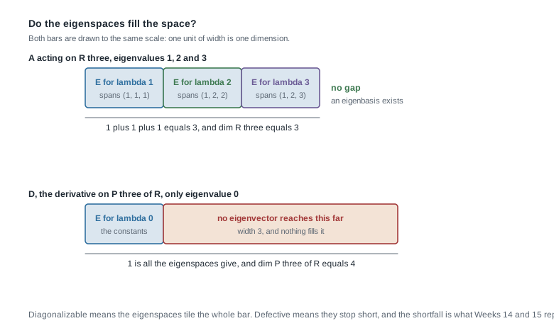
The two bars set the examples side by side at one scale. The upper bar is the \(3 \times 3\) matrix above, three eigenspaces of dimension one tiling a three-dimensional space with nothing left over; the lower bar is differentiation on \(P_3(\mathbb{R})\), one dimension of eigenvectors inside a four-dimensional space and a gap of width three. Diagonalizable means the bar is tiled, and the width of the gap is what Weeks 14 and 15 fill with generalized eigenvectors.

Characteristic moves the count. Over \(\mathbb{F}_3\) the entry \(3\) becomes \(0\), so the kernel grows to \(\operatorname{span}\{1, x^3\}\) and \(\operatorname{geo}(0) = 2\); over \(\mathbb{F}_2\) the entry \(2\) vanishes instead and the kernel is \(\operatorname{span}\{1, x^2\}\), again of dimension two. The gap narrows and never closes, because \(D_{\mathrm{iff}}\) is not the zero operator on \(P_3(F)\) over any field.

Algebraic against geometric multiplicity on four small operators.

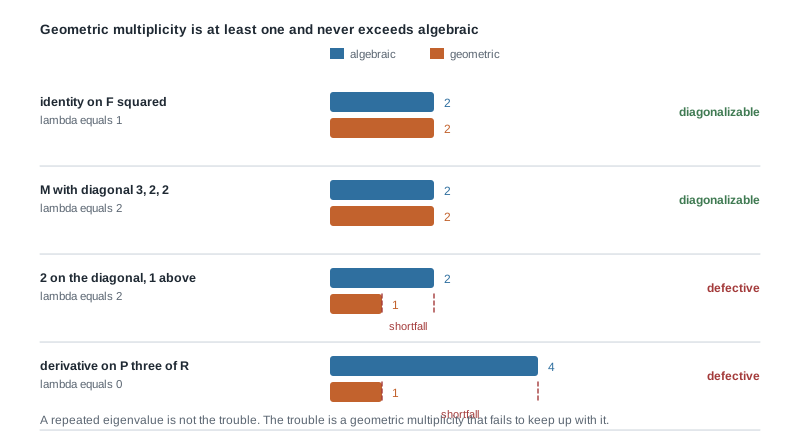
The four rows are the cases to keep in your pocket. The identity on \(F^2\) has \(\operatorname{alg}(1) = \operatorname{geo}(1) = 2\) and is already diagonal. The matrix \(M\) with columns \((3,1,1)\), \((0,2,0)\), \((0,0,2)\) is lower triangular with diagonal \(3, 2, 2\), so \(\operatorname{alg}(2) = 2\); and \(M - 2I\) has all three rows equal to \((1,0,0)\), hence rank one, so \(\operatorname{geo}(2) = 2\) and \(M\) is diagonalizable despite the repetition. The last two rows are the defective pair just examined. Repetition shows in the blue bars alone; only the orange bars decide.

The misreading to avoid

The misreading, in the words it is usually said: the matrix has a repeated eigenvalue, so it is not diagonalizable. The identity \(I_n\) refutes it in one line, with \(\operatorname{alg}(1) = n\) as repeated as an eigenvalue can be and the matrix diagonal already; the bar chart’s second row refutes it for a matrix that is not diagonal to begin with.

A repeated eigenvalue creates an opportunity to fail, not a failure. When \(\operatorname{alg}(\lambda) = 1\), the sandwich \(1 \le \operatorname{geo}(\lambda) \le \operatorname{alg}(\lambda) = 1\) leaves no room. When \(\operatorname{alg}(\lambda) = a \ge 2\), the geometric multiplicity may be anywhere from \(1\) to \(a\), and only \(\dim \ker(T - \lambda I)\) decides. The correct habit is therefore to row reduce \(A - \lambda I\), read its rank \(r\), and record \(\operatorname{geo}(\lambda) = n - r\).

Four neighbours deserve naming. The converse of the easy sufficient condition — distinct eigenvalues are needed — is false; distinct eigenvalues are sufficient and never necessary, and \(I_n\) refutes that too. The field slips out of the sentence in this matrix is diagonalizable because it has \(n\) distinct eigenvalues, which is a statement only once you say where the eigenvalues live: the quarter-turn rotation of \(\mathbb{R}^2\) has the distinct eigenvalues \(i\) and \(-i\) with eigenvectors \((1,-i)\) and \((1,i)\), neither in \(\mathbb{R}^2\), so the same array of integers is diagonalizable over \(\mathbb{C}\) and not over \(\mathbb{R}\). That rotation also kills the genuine converse of the misreading, not diagonalizable, so some eigenvalue is repeated: over \(\mathbb{R}\) it is not diagonalizable, and no eigenvalue of it is repeated anywhere, since over \(\mathbb{R}\) it has none at all and over \(\mathbb{C}\) it has the two distinct ones just named. Costliest in proofs is equal characteristic polynomials imply similar, ended by \(2I_2\) against \(\begin{pmatrix} 2 & 1 \\ 0 & 2 \end{pmatrix}\), and its improved version adding all geometric multiplicities, ended by the dimension-four pair above.

Practice on your own

These are for your own checking rather than for submission, and each is reachable with Weeks 1 through 11, apart from the single later fact that the fourth item hands you outright.

1. An invariant not on the list. Prove that \(A \sim B\) implies \(A^{\mathsf{T}} \sim B^{\mathsf{T}}\), and that \(A\) and \(A^{\mathsf{T}}\) share a characteristic polynomial. Then decide, with proof or counterexample, whether \(\operatorname{rank}(A^2)\) is a similarity invariant.
2. Multiplicities by hand. For \(A = \begin{pmatrix} 5 & -1 & 1 \\ 0 & 4 & 0 \\ 0 & 1 & 4 \end{pmatrix}\) over \(\mathbb{R}\), compute \(p_A\), find both multiplicities at each eigenvalue by row reducing \(A - \lambda I\), and decide diagonalizability. If it is diagonalizable, produce \(P\) and check \(AP = PD\) rather than inverting \(P\).
3. The field matters. Let \(A = \begin{pmatrix} 0 & 1 \\ 1 & 1 \end{pmatrix}\). Show \(p_A(t) = t^2 - t - 1\) is irreducible over \(\mathbb{Q}\), so \(A\) is not diagonalizable there, and diagonalise it over \(\mathbb{R}\). Then over \(\mathbb{F}_2\), where \(p_A(t) = t^2 + t + 1\), decide diagonalizability by testing both field elements as roots.
4. A sharper question. Let \(T\) act on a finite-dimensional \(V\) with \(\dim V = n\), and let \(\lambda \in F\) be an eigenvalue with \(\operatorname{alg}(\lambda) = 3\) and \(\operatorname{geo}(\lambda) = 2\). Granting the fact Week 14 will prove — that \(\dim \ker(T - \lambda I)^{n} = \operatorname{alg}(\lambda)\) — show that those two numbers force \(\dim \ker(T - \lambda I)^{2} = 3\) exactly. Then find the smallest \(a\) for which \(\operatorname{alg}(\lambda) = a\) and \(\operatorname{geo}(\lambda) = 2\) leave \(\dim \ker(T - \lambda I)^{2}\) undetermined, and exhibit two operators realising different values of it there.
5. Commuting and not. Exhibit two diagonalizable \(2 \times 2\) real matrices that do not commute, and confirm that no single \(P\) diagonalises both. Then exhibit two commuting matrices with at least one not diagonalizable, and name the hypothesis of the simultaneous diagonalization theorem your pair violates.

Where to read more

This page stands on its own, but a second treatment in a different voice is often what makes a theorem settle. The three addresses below are offered online at no cost by their providers; availability and licence terms are as those providers state them, and neither is confirmed here.

• MIT OpenCourseWare 18.700 Linear Algebra — a proof-based course whose eigenvalue and diagonalization material runs parallel to this week.
• Linear Algebra Done Wrong by Sergei Treil — an abstract-first text taking diagonalization and the two multiplicities in the order used here.
• MIT OpenCourseWare 18.06 Linear Algebra — the computational complement, for matrix powers on explicit numerical arrays.
• The optional Roman alignment for this week is the chapter on eigenvalues and eigenvectors, in the sections on similarity of matrices and on diagonalization. That text is an optional reference: a borrowed or library copy suffices, purchase is required for nothing on this site, and nothing from it is reproduced here.
• Course pages: the notes overview, the syllabus, the schedule, and the resources page. The learning management system remains authoritative for section logistics and graded details.

Where this goes next

You now hold a complete test for the simplest similarity class: an operator on a finite-dimensional space over \(F\) is diagonalizable exactly when \(p_T\) splits over \(F\) and every eigenvalue’s geometric multiplicity equals its algebraic one, and when the test passes the columns of \(P\) are the eigenbasis and \(D\) lists the eigenvalues in matching order. It can fail on splitting, which is a statement about \(F\) rather than about the operator, and it can fail on the multiplicities, which no change of field repairs.

Week 12 attacks the first failure with a large class for which the test can never fail: self-adjoint operators on a finite-dimensional inner product space, whose matrices relative to an orthonormal basis are the real symmetric and complex Hermitian ones. The spectral theorem promises those an orthonormal basis of eigenvectors, so the eigenvectors come out perpendicular rather than merely independent, and the apparatus of Weeks 5 through 9 is what proves it. Weeks 13 through 15 attack the second failure, with the minimal polynomial as the sharper test, generalized eigenvectors filling the gap the bar chart showed, and Jordan canonical form as the complete classification over an algebraically closed field. To look back: Week 10 carries the eigenvalues this page rests on, Week 4 the change-of-basis law that made similarity a definition, and the notes index and course home page list what is here.