Week 4 — Isomorphism, matrix representation, and change of basis

Where this week starts

Three weeks of deliberate abstinence are over. Week 1 built vector spaces over a field \(F\) and their subspaces; Week 2 produced dimension and proved it well defined; Week 3 introduced linear maps, showed \(\ker T\) and \(\operatorname{im} T\) are subspaces, proved rank-nullity for a finite-dimensional domain, and factored a map through a quotient. None of that mentioned a matrix. The silence was deliberate: matrices were the thing you already had, and the theory had to stand before leaning on them again.

This week they come back from the other side. Choose an ordered basis of the domain, choose one of the codomain, and a linear map becomes an array of scalars. The array is not the map; it is what the map looks like after two choices, and different choices give different arrays for the same map. Holding both facts at once — the array is useful, the array is contingent — is the work of the week.

Two things Week 3 left open are settled here. You have computed rank by row reducing since your undergraduate course, while rank-nullity was stated about a map; the two ranks agree because a matrix is a map read through a pair of coordinate isomorphisms, and an isomorphism cannot change the dimension of an image. And Week 3 produced an isomorphism \(V / \ker T \cong \operatorname{im} T\) without asking what one costs: exactly one ordered basis worth of choice.

By the end, two questions should fire whenever a matrix appears. Which pair of bases is this the matrix with respect to? And would the feature I am about to use survive a different choice? The transformation laws \(A \mapsto QAP^{-1}\) and \(A \mapsto PAP^{-1}\) are the precise form of the second question, and the gap between them is where the rest of the course begins.

Why this matters beyond the definition

Here is the mistake this material exists to prevent. Somebody computes the matrix of an operator in a convenient basis, notices that it is symmetric, and reports a conclusion about the operator. Take \(T(a, b) = (b, a)\) on \(\mathbb{R}^2\). In the standard basis its matrix is \(\begin{pmatrix} 0 & 1 \\ 1 & 0 \end{pmatrix}\), which is symmetric; in the ordered basis \(((1,0), (1,1))\) the same operator has matrix \(\begin{pmatrix} -1 & 0 \\ 1 & 1 \end{pmatrix}\), which is not. Symmetry of the array was a property of \(T\) together with a basis. Rank and trace were not: both arrays report rank \(2\) and trace \(0\).

The second stake does more damage. Because every \(n\)-dimensional space over \(F\) is isomorphic to \(F^n\), it is tempting to treat an abstract space as though it simply were \(F^n\). But \(F^n\) carries structure the abstract space does not: its elements have entries, its standard basis is singled out, its coordinates come in an order. A proof that quietly identifies \(V\) with \(F^n\) and then appeals to any of that has smuggled in a choice, and a statement depending on that choice is not a theorem about \(V\).

What you will be able to do

• State what an isomorphism of vector spaces is, and prove that the inverse of a bijective linear map is linear.
• Prove that finite-dimensional \(V\) and \(W\) over the same \(F\) are isomorphic exactly when \(\dim V = \dim W\), and say in what sense the isomorphism is not canonical.
• Construct \([T]_{\mathcal{C} \leftarrow \mathcal{B}}\) column by column and prove the identity \([Tv]_{\mathcal{C}} = [T]_{\mathcal{C} \leftarrow \mathcal{B}} [v]_{\mathcal{B}}\) that defines it.
• Derive matrix multiplication from composition of linear maps, with the middle basis matched.
• Compute a change-of-basis matrix and its inverse, and move the matrix of an operator between bases.
• Decide whether two matrices are equivalent, whether they are similar, and exhibit an invariant separating a pair that is one but not the other.

Terms and notation worth fixing

Symbol or term	What it means on this page
\(\mathcal{B} = (v_1, \dots, v_n)\)	an ordered basis: a basis with a chosen listing of its members
\([v]_{\mathcal{B}}\)	the coordinate column of \(v\): the unique \(a_1, \dots, a_n\) with \(v = a_1v_1 + \dots + a_nv_n\)
\([T]_{\mathcal{C} \leftarrow \mathcal{B}}\)	the matrix consuming \(\mathcal{B}\)-coordinates and producing \(\mathcal{C}\)-coordinates; read the subscript right to left
\(P_{\mathcal{C} \leftarrow \mathcal{B}}\)	the change-of-basis matrix \([\operatorname{id}_V]_{\mathcal{C} \leftarrow \mathcal{B}}\)
isomorphism, \(V \cong W\)	a bijective linear map, and the relation of having one
\(\mathcal{L}(V, W)\)	all linear maps \(V \to W\), itself a vector space; \(\mathcal{L}(V)\) when \(W = V\)
equivalent matrices	same shape, \(B = QAR\) with \(Q\) and \(R\) invertible
similar matrices	square, \(B = P^{-1}AP\) with \(P\) invertible
\(I_r\)	the \(r \times r\) identity, used as a block inside a larger array

Isomorphism, and the choice hidden inside it

An isomorphism is a linear map that is also a bijection. Note how little that asks: it does not require the inverse to be linear, and it never mentions bases, dimension, or coordinates. Yet in finite dimensions the relation turns out to be controlled entirely by one integer, and the gap between that fact and its naive reading is the most important thing on this page.

Bijective linear maps and their inverses

Definition. For \(V\) and \(W\) over the same field \(F\), a map \(T \in \mathcal{L}(V, W)\) is an isomorphism when it is bijective, and \(V \cong W\) means some isomorphism \(V \to W\) exists.

Proposition. If \(T \colon V \to W\) is a bijective linear map, its set-theoretic inverse \(T^{-1}\) is linear.

Argument. Let \(w_1, w_2 \in W\) and \(a \in F\), and put \(u_i = T^{-1}(w_i)\). Linearity of \(T\) gives \(T(u_1 + a u_2) = w_1 + a w_2\). Applying \(T^{-1}\) to both sides yields \(u_1 + a u_2 = T^{-1}(w_1 + a w_2)\), which is exactly \(T^{-1}(w_1 + a w_2) = T^{-1}(w_1) + a\,T^{-1}(w_2)\). Additivity and homogeneity are both contained in that identity, so \(T^{-1}\) is linear. Nothing used finite-dimensionality or a basis.

Three bookkeeping facts follow and get used silently. The identity map is an isomorphism, the proposition supplies \(W \cong V\) from \(V \cong W\), and a composition of bijective linear maps is bijective and linear. So \(\cong\) is an equivalence relation, and its classes are worth asking about.

Dimension is the complete invariant

Lemma. If \(T \colon V \to W\) is an isomorphism and \((v_1, \dots, v_n)\) is a basis of \(V\), then \((Tv_1, \dots, Tv_n)\) is a basis of \(W\).

Argument. Independence: if \(\sum_i a_i Tv_i = 0\) then \(T(\sum_i a_i v_i) = 0\), so \(\sum_i a_i v_i \in \ker T = \{0\}\) by injectivity, so every \(a_i = 0\) by independence of the \(v_i\). Spanning: given \(w \in W\), surjectivity supplies \(v\) with \(Tv = w\); write \(v = \sum_i a_i v_i\) and apply \(T\).

Theorem. Let \(V\) and \(W\) be finite-dimensional over the same field \(F\). Then \(V \cong W\) if and only if \(\dim V = \dim W\).

Argument. If \(V \cong W\), the lemma carries a basis of \(V\) to a basis of \(W\) with the same number of members, and dimension is well defined by Week 2, so the dimensions agree. Conversely, if \(\dim V = \dim W = n\), choose ordered bases \(\mathcal{B} = (v_1, \dots, v_n)\) and \(\mathcal{C} = (w_1, \dots, w_n)\). Week 3 supplies exactly one linear \(T\) with \(Tv_i = w_i\). Its image is a subspace containing the spanning set \(\{w_1, \dots, w_n\}\), so \(T\) is surjective; and \(T(\sum_i a_i v_i) = \sum_i a_i w_i = 0\) forces every \(a_i = 0\) by independence, so \(\ker T = \{0\}\) and \(T\) is injective.

Corollary. Every \(n\)-dimensional space over \(F\) is isomorphic to \(F^n\), by the theorem with \(W = F^n\).

Now the caveat, which matters more than the theorem. The converse direction did not produce an isomorphism; it produced one for each pair of ordered bases fed to it, and had nothing to say about which pair to feed it. No space hands you an isomorphism onto \(F^n\) for free — you pick, and the picking is exactly an ordered basis. Counting makes this concrete. A two-dimensional space over \(\mathbb{F}_2\) has four vectors; an ordered basis is a first vector chosen from the three nonzero ones and a second from the two outside the span of the first, so there are \(3 \cdot 2 = 6\) ordered bases and six different isomorphisms onto \(\mathbb{F}_2^2\). None is distinguished.

The field is part of the statement too. The complex numbers form a space over \(\mathbb{C}\) with \(\dim_{\mathbb{C}} \mathbb{C} = 1\) and a space over \(\mathbb{R}\) with \(\dim_{\mathbb{R}} \mathbb{C} = 2\), the latter because \((1, i)\) is an \(\mathbb{R}\)-basis. So \(\mathbb{C} \cong \mathbb{R}^2\) as real spaces, while \(\mathbb{R}^2\) is not a complex space at all until somebody says how \(i\) acts on it.

Coordinates, and why the basis must be ordered

Fix an ordered basis \(\mathcal{B} = (v_1, \dots, v_n)\) of \(V\). Every \(v\) has an expression \(v = a_1v_1 + \dots + a_nv_n\) because \(\mathcal{B}\) spans, and only one because \(\mathcal{B}\) is independent: two expressions for \(v\) would subtract to a vanishing combination whose coefficients are their differences. Define the coordinate map \[[\;\cdot\;]_{\mathcal{B}} \colon V \to F^n, \qquad [v]_{\mathcal{B}} = \begin{pmatrix} a_1 \\ \vdots \\ a_n \end{pmatrix} .\] It is linear, since expanding \(u + \lambda v\) and invoking uniqueness shows its coefficients are the corresponding sums and multiples; it is bijective, since \((a_1, \dots, a_n) \mapsto \sum_i a_i v_i\) inverts it on both sides. So it is an isomorphism \(V \to F^n\), and it is the isomorphism the corollary was really about.

The order is not decoration. Reordering \(\mathcal{B}\) to \((v_2, v_1, v_3, \dots, v_n)\) gives a different isomorphism onto the same \(F^n\), one that swaps the first two entries of every column; a single unordered basis of \(n\) vectors carries \(n!\) such maps. That is why this block writes an ordered basis as a tuple. In \(P_3(F)\), the polynomials over \(F\) of degree at most three, the standard ordered basis is \((1, x, x^2, x^3)\) and \(\dim P_3(F) = 4\) — four, because the subscript bounds the degree and the constants are in there too.

Putting bases on a map and reading off a matrix

Let \(T \colon V \to W\) be linear with \(\dim V = n\) and \(\dim W = m\), both finite, and fix ordered bases \(\mathcal{B} = (v_1, \dots, v_n)\) of \(V\) and \(\mathcal{C} = (w_1, \dots, w_m)\) of \(W\). Two coordinate isomorphisms are now in play, one at each end. Squeezing \(T\) between them produces a map \(F^n \to F^m\), that map turns out to be multiplication by a matrix, and finding the matrix is a matter of asking what \(T\) does to the basis you started from.

The defining identity of the matrix of a map

Definition. The matrix of \(T\) relative to \(\mathcal{B}\) and \(\mathcal{C}\), written \([T]_{\mathcal{C} \leftarrow \mathcal{B}}\), is the \(m \times n\) array over \(F\) whose \(j\)-th column is \([Tv_j]_{\mathcal{C}}\); equivalently its entries \(A_{ij}\) satisfy \(Tv_j = \sum_{i=1}^{m} A_{ij} w_i\). Read the subscript right to left: \(\mathcal{B}\)-coordinates in on the right, \(\mathcal{C}\)-coordinates out on the left.

Theorem. \([Tv]_{\mathcal{C}} = [T]_{\mathcal{C} \leftarrow \mathcal{B}}\, [v]_{\mathcal{B}}\) for every \(v \in V\), and \([T]_{\mathcal{C} \leftarrow \mathcal{B}}\) is the only \(m \times n\) matrix with that property.

Argument. Write \(A = [T]_{\mathcal{C} \leftarrow \mathcal{B}}\) and \(v = \sum_j a_j v_j\). Linearity of \(T\) gives \(Tv = \sum_j a_j Tv_j\), and linearity of the coordinate map gives \[[Tv]_{\mathcal{C}} = \sum_{j=1}^{n} a_j\, [Tv_j]_{\mathcal{C}} = \sum_{j=1}^{n} a_j \cdot (\text{$j$-th column of } A) = A\,[v]_{\mathcal{B}} ,\] the last step being the definition of a matrix acting on a column. For uniqueness, suppose \(M[v]_{\mathcal{B}} = A[v]_{\mathcal{B}}\) for all \(v\); taking \(v = v_j\) makes \([v_j]_{\mathcal{B}}\) the \(j\)-th standard column, and multiplying by it returns the \(j\)-th column, so \(M\) and \(A\) agree column by column.

The matrix of a map turns a square of maps into an identity you can check.

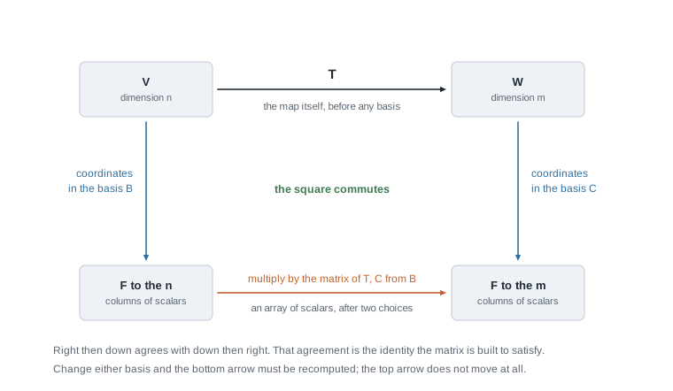
The square is the theorem in one picture: the top arrow is the map, the side arrows are the coordinate isomorphisms attached to \(\mathcal{B}\) and \(\mathcal{C}\), and the bottom arrow is multiplication by the array. Saying the square commutes says exactly that \([Tv]_{\mathcal{C}} = A[v]_{\mathcal{B}}\). Notice what else it shows: replace either side arrow and the bottom arrow must be recomputed to keep the square closed, while the top arrow never moves.

Composition is where matrix multiplication comes from

Theorem. Let \(V\), \(W\), \(Z\) be finite-dimensional over \(F\) with ordered bases \(\mathcal{B}\), \(\mathcal{C}\), \(\mathcal{D}\), and let \(T \colon V \to W\), \(S \colon W \to Z\) be linear. Then \([S \circ T]_{\mathcal{D} \leftarrow \mathcal{B}} = [S]_{\mathcal{D} \leftarrow \mathcal{C}}\, [T]_{\mathcal{C} \leftarrow \mathcal{B}}\).

Argument. For every \(v\), apply the defining identity three times: \[[(S \circ T)v]_{\mathcal{D}} = [S(Tv)]_{\mathcal{D}} = [S]_{\mathcal{D} \leftarrow \mathcal{C}}\,[Tv]_{\mathcal{C}} = [S]_{\mathcal{D} \leftarrow \mathcal{C}}\,[T]_{\mathcal{C} \leftarrow \mathcal{B}}\,[v]_{\mathcal{B}} .\] So that product has the property characterising \([S \circ T]_{\mathcal{D} \leftarrow \mathcal{B}}\), and uniqueness finishes it.

This is the honest origin of the rule for multiplying matrices. An entry of a product is a sum over the middle index because composing runs a vector through the middle space and expands it in the middle basis on the way. The two inner subscripts must be the same \(\mathcal{C}\) — outputs of \(T\) written in the basis used to read inputs of \(S\) — which is why the shapes must match.

The space of maps and the space of matrices

Give \(\mathcal{L}(V, W)\) the pointwise operations \((S + T)(v) = S(v) + T(v)\) and \((\lambda T)(v) = \lambda\,T(v)\). Both results are linear by a two-line check, and the Week 1 axioms hold because they hold pointwise in \(W\), with the zero map as additive identity. So \(\mathcal{L}(V, W)\) is a vector space over \(F\), and we can ask how big it is.

Theorem. If \(\dim V = n\) and \(\dim W = m\) are finite, then \(\dim \mathcal{L}(V, W) = mn\).

Argument. Fix \(\mathcal{B}\) and \(\mathcal{C}\) and let \(\Phi(T) = [T]_{\mathcal{C} \leftarrow \mathcal{B}}\), a map \(\mathcal{L}(V, W) \to M_{m \times n}(F)\). It is linear, since the \(j\)-th column of \(\Phi(S + \lambda T)\) is \([Sv_j]_{\mathcal{C}} + \lambda[Tv_j]_{\mathcal{C}}\). It is injective, since a map with zero matrix kills every \(v_j\) and is the zero map by determination on a basis. It is surjective, since determination on a basis produces \(T\) with \(Tv_j = \sum_i A_{ij}w_i\) for any given array \(A\). So \(\Phi\) is an isomorphism and \(\dim \mathcal{L}(V, W) = \dim M_{m \times n}(F) = mn\), the last count because the arrays with a single \(1\) and zeros elsewhere form a basis. So \(\dim \mathcal{L}(P_3(F)) = 16\) and \(\dim \mathcal{L}(\mathbb{R}^3, \mathbb{R}^2) = 6\).

Change of basis and the two transformation laws

Apply the definition to the identity operator with different bases at the two ends. For ordered bases \(\mathcal{B}\), \(\mathcal{C}\) of one space \(V\), set \(P_{\mathcal{C} \leftarrow \mathcal{B}} = [\operatorname{id}_V]_{\mathcal{C} \leftarrow \mathcal{B}}\), whose \(j\)-th column is \([v_j]_{\mathcal{C}}\). The defining identity reads \([v]_{\mathcal{C}} = P_{\mathcal{C} \leftarrow \mathcal{B}}[v]_{\mathcal{B}}\): it rewrites a \(\mathcal{B}\)-column as the \(\mathcal{C}\)-column of the same vector and moves no vectors at all. Composing \(\operatorname{id}\) with \(\operatorname{id}\), \[P_{\mathcal{B} \leftarrow \mathcal{C}}\, P_{\mathcal{C} \leftarrow \mathcal{B}} = [\operatorname{id}_V]_{\mathcal{B} \leftarrow \mathcal{B}} = I_n ,\] and symmetrically, so \(P_{\mathcal{C} \leftarrow \mathcal{B}}\) is invertible with inverse \(P_{\mathcal{B} \leftarrow \mathcal{C}}\).

Two coordinate systems on one space, joined by the change-of-basis matrix.

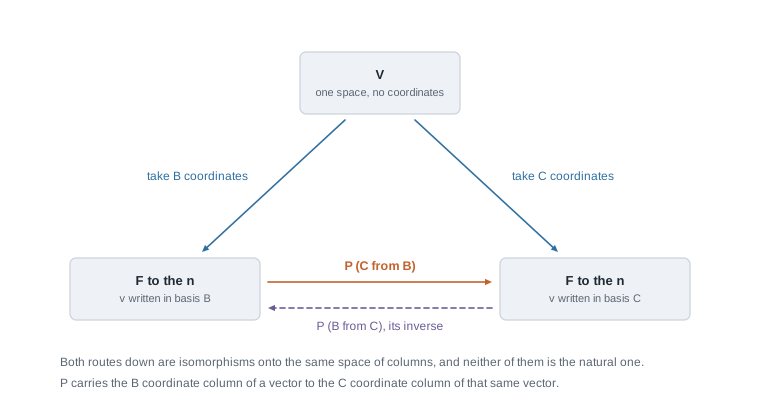
The triangle holds one space and two ways of writing its vectors as columns: the descending arrows are the coordinate isomorphisms, the horizontal arrows are \(P\) and \(P^{-1}\), translating between column languages without touching the space at the apex. A change of basis is a dictionary, not an operation performed on vectors.

Now push a map through. Let \(T \colon V \to W\), with \(\mathcal{B}, \mathcal{B}'\) ordered bases of \(V\) and \(\mathcal{C}, \mathcal{C}'\) of \(W\). Writing \(T = \operatorname{id}_W \circ\, T \circ \operatorname{id}_V\) and composing matrices, \[[T]_{\mathcal{C}' \leftarrow \mathcal{B}'} = P_{\mathcal{C}' \leftarrow \mathcal{C}}\; [T]_{\mathcal{C} \leftarrow \mathcal{B}}\; P_{\mathcal{B} \leftarrow \mathcal{B}'} = Q\,A\,P^{-1},\] with \(A = [T]_{\mathcal{C} \leftarrow \mathcal{B}}\), \(Q = P_{\mathcal{C}' \leftarrow \mathcal{C}}\), and \(P = P_{\mathcal{B}' \leftarrow \mathcal{B}}\), so \(P_{\mathcal{B} \leftarrow \mathcal{B}'} = P^{-1}\). Two invertible matrices chosen independently, one on each side: this relation is matrix equivalence. If \(W = V\) and one basis must serve both ends — as it must, if the operator is to be composed with itself — then \(\mathcal{C} = \mathcal{B}\), \(\mathcal{C}' = \mathcal{B}'\), so \(Q = P\) and the law collapses to \(A \mapsto PAP^{-1}\). That relation is similarity.

Equivalence, similarity, and the rank normal form

Theorem (rank normal form). Let \(T \colon V \to W\) be linear with \(\dim V = n\), \(\dim W = m\) finite and \(\operatorname{rank} T = r\). Then there are ordered bases \(\mathcal{B}\) of \(V\) and \(\mathcal{C}\) of \(W\) with \([T]_{\mathcal{C} \leftarrow \mathcal{B}} = \begin{pmatrix} I_r & 0 \\ 0 & 0 \end{pmatrix}\), the \(m \times n\) array with an \(r \times r\) identity block upper left and zeros elsewhere.

Argument. Rank-nullity gives \(\dim \ker T = n - r\). Take a basis \((u_{r+1}, \dots, u_n)\) of \(\ker T\), extend to a basis of \(V\), and order the added vectors first: \(\mathcal{B} = (u_1, \dots, u_n)\). The Week 3 proof shows \((Tu_1, \dots, Tu_r)\) is a basis of \(\operatorname{im} T\); extend it to an ordered basis \(\mathcal{C}\) of \(W\) with \(m - r\) further vectors. For \(j \le r\), \(Tu_j\) is the \(j\)-th member of \(\mathcal{C}\), so column \(j\) is the \(j\)-th standard column; for \(j > r\), \(Tu_j = 0\), so the remaining columns vanish.

Every rank-r map reaches the same block shape once the bases are chosen for it.

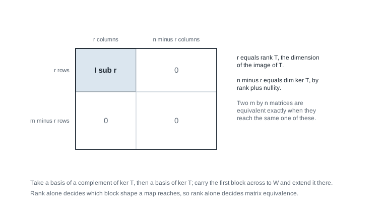
The block picture makes rank-nullity visible as a shape: the \(r\) left columns are what a complement of the kernel contributes, the \(n - r\) right columns are the kernel, the top \(r\) rows are the image, the bottom \(m - r\) rows are everything in \(W\) the map never reaches. Two consequences follow. First, \(\operatorname{rank}(QAR) = \operatorname{rank} A\) for invertible \(Q\) and \(R\), since those are matrices of isomorphisms and an isomorphism changes no image dimension. Second, two \(m \times n\) matrices are equivalent if and only if their ranks agree: each is equivalent to the normal form of its own rank, and equivalence is symmetric and transitive.

Similarity is strictly finer. Every similar pair is equivalent, since \(P^{-1}AP\) has the shape \(QAR\). But equal rank no longer suffices, because similarity may not change the two bases independently, and the second worked example exhibits two rank-one matrices that no single \(P\) connects. Cataloguing similarity classes is the business of the rest of the course, with eigenvalues, characteristic polynomials, diagonalization and Jordan canonical form as the tools; this week only establishes that the question is real.

Worked example — the shift on cubic polynomials in two bases

Work over \(\mathbb{R}\) with \(V = P_3(\mathbb{R})\), so \(\dim V = 4\), and let \((Tp)(x) = p(x + 1)\). This is linear, because substitution respects sums and scalar multiples, and it preserves degree, so it maps \(V\) into \(V\). The task: compute its matrix in two bases, produce the change-of-basis matrix, and verify the similarity relation by multiplying out.

Step 1. The standard basis. Take \(\mathcal{B} = (1, x, x^2, x^3)\) and expand by the binomial theorem: \[T(1) = 1, \quad T(x) = 1 + x, \quad T(x^2) = 1 + 2x + x^2, \quad T(x^3) = 1 + 3x + 3x^2 + x^3 .\] Each coefficient list is a column, in that order, so \[A = [T]_{\mathcal{B} \leftarrow \mathcal{B}} = \begin{pmatrix} 1 & 1 & 1 & 1 \\ 0 & 1 & 2 & 3 \\ 0 & 0 & 1 & 3 \\ 0 & 0 & 0 & 1 \end{pmatrix} .\]

Step 2. A second basis. Let \(\mathcal{C} = (c_0, c_1, c_2, c_3)\) with \(c_0 = 1\), \(c_1 = x\), \(c_2 = x(x-1)\), \(c_3 = x(x-1)(x-2)\). Their degrees are \(0, 1, 2, 3\), so they are independent, and four independent vectors in a four-dimensional space form a basis by Week 2. Substituting: \[\begin{aligned} Tc_0 &= 1 = c_0, \\ Tc_1 &= x + 1 = c_1 + c_0, \\ Tc_2 &= (x+1)x = x^2 + x = (x^2 - x) + 2x = c_2 + 2c_1, \\ Tc_3 &= (x+1)x(x-1) = x^3 - x = (x^3 - 3x^2 + 2x) + (3x^2 - 3x) = c_3 + 3c_2 . \end{aligned}\] Each image is one basis vector plus a multiple of the previous one, so \[B = [T]_{\mathcal{C} \leftarrow \mathcal{C}} = \begin{pmatrix} 1 & 1 & 0 & 0 \\ 0 & 1 & 2 & 0 \\ 0 & 0 & 1 & 3 \\ 0 & 0 & 0 & 1 \end{pmatrix} .\] The same operator, and a visibly simpler array: three entries above the diagonal have been cleared by nothing but a change of basis.

Step 3. The change-of-basis matrices. The columns of \(P = P_{\mathcal{B} \leftarrow \mathcal{C}}\) are the \(\mathcal{B}\)-coordinates of the members of \(\mathcal{C}\). Expanding, \(c_2 = -x + x^2\) and \(c_3 = 2x - 3x^2 + x^3\), so \[P = P_{\mathcal{B} \leftarrow \mathcal{C}} = \begin{pmatrix} 1 & 0 & 0 & 0 \\ 0 & 1 & -1 & 2 \\ 0 & 0 & 1 & -3 \\ 0 & 0 & 0 & 1 \end{pmatrix}, \qquad P^{-1} = P_{\mathcal{C} \leftarrow \mathcal{B}} = \begin{pmatrix} 1 & 0 & 0 & 0 \\ 0 & 1 & 1 & 1 \\ 0 & 0 & 1 & 3 \\ 0 & 0 & 0 & 1 \end{pmatrix} .\] The columns of \(P^{-1}\) are the \(\mathcal{C}\)-coordinates of \(1, x, x^2, x^3\): indeed \(x^2 = c_2 + c_1\) and \(x^3 = c_3 + 3c_2 + c_1\), both checkable by expanding. Multiplying confirms the inverse: row two of \(P\) is \((0, 1, -1, 2)\), and against the columns of \(P^{-1}\) it gives \(0\), \(1\), \(1 - 1 = 0\), \(1 - 3 + 2 = 0\); row three is \((0, 0, 1, -3)\) and gives \(0\), \(0\), \(1\), \(3 - 3 = 0\); rows one and four are immediate.

Step 4. Verify the similarity relation. The transformation law for an operator says \(A = P B P^{-1}\) with \(P = P_{\mathcal{B} \leftarrow \mathcal{C}}\). Multiply in two stages. First \[PB = \begin{pmatrix} 1 & 1 & 0 & 0 \\ 0 & 1 & 1 & -1 \\ 0 & 0 & 1 & 0 \\ 0 & 0 & 0 & 1 \end{pmatrix},\] whose second row comes from \((0,1,-1,2)\) against the columns of \(B\): \(0\), then \(1\), then \(2 - 1 = 1\), then \(-3 + 2 = -1\). Then multiply on the right by \(P^{-1}\), whose columns are \((1,0,0,0)\), \((0,1,0,0)\), \((0,1,1,0)\), \((0,1,3,1)\). Row one of \(PB\) is \((1,1,0,0)\) and produces \(1, 1, 1, 1\); row two is \((0,1,1,-1)\) and produces \(0\), \(1\), \(1 + 1 = 2\), \(1 + 3 - 1 = 3\); row three is \((0,0,1,0)\) and produces \(0, 0, 1, 3\); row four produces \(0, 0, 0, 1\). That is exactly \(A\).

Step 5. A coordinate check on one vector. Take \(p = x^3\). Then \([p]_{\mathcal{B}} = (0,0,0,1)^{\mathsf{T}}\) and \(A[p]_{\mathcal{B}}\) is the fourth column \((1,3,3,1)^{\mathsf{T}}\), reading back as \(1 + 3x + 3x^2 + x^3 = (x+1)^3\). And \([p]_{\mathcal{C}} = (0,1,3,1)^{\mathsf{T}}\) with \(B[p]_{\mathcal{C}} = (1, 7, 6, 1)^{\mathsf{T}}\), reading back as \(c_0 + 7c_1 + 6c_2 + c_3 = 1 + 7x + 6(x^2 - x) + (x^3 - 3x^2 + 2x) = 1 + 3x + 3x^2 + x^3\). One polynomial, two arrays, same image.

So \(A\) and \(B\) are two records of one operator, tied by a dictionary, and the tie can be checked with arithmetic alone. What this does not establish is that either array is the operator, or that \(B\) is the simplest array available. One remark on the field: every entry of \(P\) and \(P^{-1}\) is an integer and \(\det P = 1\), so \(A = PBP^{-1}\) holds verbatim over any \(F\) once the numbers are read in \(F\). Over \(\mathbb{F}_3\) the entries equal to \(3\) become \(0\) and both arrays change shape, yet the relation between them does not.

The same reasoning, transferred

Run the same steps on \(\mathbb{R}^2\), where the products fit on one line. Let \(T(a, b) = (a + b, b)\), the shear sliding each point horizontally by its own height, and let \(\mathcal{E} = (e_1, e_2)\) be standard. Then \(Te_1 = e_1\) and \(Te_2 = (1,1) = e_1 + e_2\), so \(A = \begin{pmatrix} 1 & 1 \\ 0 & 1 \end{pmatrix}\). Take the skewed ordered basis \(\mathcal{F} = (f_1, f_2)\) with \(f_1 = (1,1)\), \(f_2 = (0,1)\). Then \(Tf_1 = (2,1) = 2f_1 - f_2\) and \(Tf_2 = (1,1) = f_1\), so \[[T]_{\mathcal{F} \leftarrow \mathcal{F}} = \begin{pmatrix} 2 & 1 \\ -1 & 0 \end{pmatrix}, \qquad P = P_{\mathcal{E} \leftarrow \mathcal{F}} = \begin{pmatrix} 1 & 0 \\ 1 & 1 \end{pmatrix}, \qquad P^{-1} = \begin{pmatrix} 1 & 0 \\ -1 & 1 \end{pmatrix} .\] Check: \(P\begin{pmatrix} 2 & 1 \\ -1 & 0 \end{pmatrix} = \begin{pmatrix} 2 & 1 \\ 1 & 1 \end{pmatrix}\), then \(\begin{pmatrix} 2 & 1 \\ 1 & 1 \end{pmatrix}P^{-1} = \begin{pmatrix} 1 & 1 \\ 0 & 1 \end{pmatrix} = A\). What stayed the same: the column-by-column definition, the construction of \(P\) from coordinates of the new basis in the old, and the law. What changed: the space, the dimension, and the direction of the simplification, since the second array is uglier and nothing promises a change of basis will improve matters. Two numbers did not move: both arrays have trace \(2\) and determinant \(1\).

Second worked example — equal rank, and still not similar

Let \(F\) be any field and work in \(M_2(F)\), read as matrices of operators on \(F^2\) in the standard basis. Put \[N = \begin{pmatrix} 0 & 1 \\ 0 & 0 \end{pmatrix}, \qquad E = \begin{pmatrix} 1 & 0 \\ 0 & 0 \end{pmatrix} .\] Both have rank one: the columns of each span the line through \((1,0)\), and neither is zero. By the classification above they are equivalent, and the equivalence needs no theory. Let \(R = \begin{pmatrix} 0 & 1 \\ 1 & 0 \end{pmatrix}\), invertible with \(R^2 = I_2\). Then \(ER = N\), so \(N = I_2 \cdot E \cdot R\) has the form \(QER\) with both outer factors invertible: \(E\) and \(N\) are one map read with different bases at the two ends.

Now show no single \(P\) works at both ends. Three arguments live inside this block.

Squaring. \(E^2 = E\) while \(N^2 = 0 \ne N\). If \(N = P^{-1}EP\) then \(N^2 = P^{-1}EPP^{-1}EP = P^{-1}E^2P = P^{-1}EP = N\), contradicting \(N^2 = 0\) with \(N \ne 0\). So similarity preserves \(A^2 = A\); equivalence plainly does not, since \(E\) has the property and \(N\) does not.

Nullity of a shifted matrix. For any \(\lambda \in F\) and invertible \(P\), \(P^{-1}AP - \lambda I = P^{-1}(A - \lambda I)P\), so the two kernels have equal dimension, multiplication by \(P\) carrying one bijectively onto the other. Take \(\lambda = 1\). Then \(E - I = \begin{pmatrix} 0 & 0 \\ 0 & -1 \end{pmatrix}\) has rank one, so rank-nullity gives its kernel dimension one; while \(N - I = \begin{pmatrix} -1 & 1 \\ 0 & -1 \end{pmatrix}\) has rank two, since row reduction leaves two nonzero rows, so its kernel has dimension zero. One and zero differ, so \(E\) and \(N\) are not similar.

Trace. Granting \(\operatorname{tr}(XY) = \operatorname{tr}(YX)\), a direct computation on the double sum, \(\operatorname{tr}(P^{-1}AP) = \operatorname{tr}(APP^{-1}) = \operatorname{tr} A\), so trace is a similarity invariant; here \(\operatorname{tr} E = 1\) and \(\operatorname{tr} N = 0\). It is not an equivalence invariant, since \(N\) and \(E\) have equal rank.

What matrix equivalence and similarity are each allowed to change.

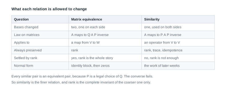
The table gathers the contrast this example has made concrete. Down one column: two independent basis changes, maps between two spaces, rank preserved, rank sufficient. Down the other: one basis change used at both ends, operators, rank and trace and idempotence preserved, rank insufficient. The difference is the loss of one degree of freedom, and that loss is what makes similarity carry information. Note that every step above used only \(1 \ne 0\) in \(F\), so the conclusion holds over \(\mathbb{F}_2\) too, where \(-1 = 1\) makes the arrays look different but changes neither rank.

The misreading to avoid

The misreading: every \(n\)-dimensional space over \(F\) is \(F^n\), so I may as well work in \(F^n\) and stop worrying about the abstract space. The first clause is a real theorem read too fast. What is true is that every such space is isomorphic to \(F^n\), and that an isomorphism appears the moment you choose an ordered basis. What is false is that the space is \(F^n\), or that one identification is preferred. \(P_3(\mathbb{R})\) has no first coordinate until somebody says which polynomial is \(v_1\); in the worked example the same operator had matrix \(A\) under one choice and \(B\) under another, with nothing available to single out either.

A useful diagnostic: if you can state your claim without mentioning a basis, it is a claim about the space or the map, and coordinates are a legitimate way to prove it. If you cannot — if the claim mentions entries, or the first coordinate, or symmetry of an array — then coordinates are part of the statement rather than a proof technique, and the choice must be carried explicitly. The swap operator at the top of this page is the small version: symmetric in one basis, not in another, so “symmetric” is not yet a property of an operator.

The second misreading is that similar and equivalent name the same idea. Equivalence is what you get when bases may change independently at each end, and rank is a complete invariant for it. Similarity is what remains when one basis serves both ends, and rank is nowhere near enough; the rank-one pair \(N\) and \(E\) is the smallest counterexample that works over every field — over any \(F\) with more than two elements the \(1 imes 1\) pair \((1)\) and \((2)\) already has equal rank and unequal trace — and it is worth keeping in your pocket. A slogan that helps: equivalence asks what the map does, similarity asks what it does repeatedly, since only an operator composes with itself and only similarity respects that composition.

Practice on your own

These are for your own checking rather than for submission, and each is within reach of Weeks 1 through 4.

1. Injective, surjective, bijective. Let \(\dim V = \dim W\) be finite and \(T \in \mathcal{L}(V, W)\). Prove \(T\) is injective if and only if it is surjective. Then locate the step that breaks when \(\dim V \ne \dim W\), and the step that breaks for the shift on \(F^{\mathbb{N}}\), which is injective and not surjective.
2. A second operator on \(P_3\). Let \(D\) be differentiation on \(P_3(\mathbb{R})\). Compute \([D]_{\mathcal{B} \leftarrow \mathcal{B}}\) in the standard basis, then \([D]_{\mathcal{C} \leftarrow \mathcal{C}}\) in the basis \(\mathcal{C}\) above, and reconcile the two arrays using the \(P\) computed there. Confirm both have rank three and trace zero.
3. Same rank, not similar. Produce two \(3 \times 3\) real matrices of rank two that are not similar, and prove the failure with an invariant from this page rather than by hunting for \(P\). Then produce a third rank-two matrix similar to your first, exhibiting the \(P\) that does it.
4. Counting identifications. How many ordered bases does \(\mathbb{F}_2^3\) have? Count by choosing vectors one at a time and excluding the span of what you already hold. Then say in one sentence what the count has to do with the claim that no identification is canonical.
5. Composition and the middle basis. Let \(T \colon \mathbb{R}^3 \to \mathbb{R}^2\) and \(S \colon \mathbb{R}^2 \to \mathbb{R}^4\) be linear, and suppose you hold \([T]_{\mathcal{C} \leftarrow \mathcal{B}}\) and \([S]_{\mathcal{D} \leftarrow \mathcal{C}'}\) where \(\mathcal{C}\) and \(\mathcal{C}'\) are different ordered bases of \(\mathbb{R}^2\). Write the correct product for \([S \circ T]_{\mathcal{D} \leftarrow \mathcal{B}}\), with the change-of-basis matrix in the right place and facing the right way, and state the shape of the result.

Where to read more

This page stands on its own, but a second treatment in a different voice is often what makes a theorem settle. The three addresses below are offered online at no cost by their providers; availability and licence terms are as those providers state them, and neither is confirmed here.

• MIT OpenCourseWare 18.700 Linear Algebra — a proof-based course whose treatment of linear maps, matrix representation, and change of basis runs parallel to this week.
• Linear Algebra Done Wrong by Sergei Treil — an abstract-first text whose chapter on linear transformations develops coordinates, the matrix of a map, and change of basis in the order used here.
• MIT OpenCourseWare 18.06 Linear Algebra — the computational complement, for similarity and rank exercised on explicit numerical arrays.
• The optional Roman alignment for this week is Chapter 1, in the section on ordered bases and coordinate matrices, with Chapter 2, in the sections on isomorphisms, the matrix of a linear transformation, change of basis matrices, equivalence of matrices, and similarity of matrices. That text is an optional reference: a borrowed or library copy suffices, and nothing from it is reproduced here.
• Course pages: the notes overview, the syllabus, the schedule, and the resources page. The learning management system remains authoritative for section logistics and graded details.

Where this goes next

This week closes the opening block on a question rather than a conclusion. You now know that a matrix is a map plus two choices, that changing the choices moves it by \(A \mapsto QAP^{-1}\) in general and by \(A \mapsto PAP^{-1}\) for an operator, and that rank settles the first relation completely and the second not at all. What does settle similarity is the question the remainder of the course is organised around, and the route there runs through geometry first.

Week 5, on inner products, norms, and the geometry they impose, opens that route: it equips a space with an inner product, reads a norm off it, and proves the Cauchy-Schwarz and triangle inequalities that make orthogonality a usable notion. Weeks 5 through 9 develop that geometry — orthogonal sets and projections, and bilinear and quadratic forms — supplying the length and angle Weeks 1 through 4 deliberately did without; Weeks 10 through 15 then return to the similarity question with eigenvalues, diagonalization, the spectral theorem for symmetric and Hermitian matrices, and the Jordan canonical form, which describes similarity classes as completely as the rank normal form described equivalence classes. To look back instead: Week 3 carries the rank-nullity theorem and the quotient constructions this week rests on, and the notes index and course home page list what is here.