Week 10 — Eigenvalues, eigenvectors, and invariant subspaces
Where this week starts
Week 4 closed the opening block with a question rather than a theorem: two matrices representing one operator in different bases are related by \(A \mapsto PAP^{-1}\), and rank — which settled matrix equivalence completely — settles nothing about similarity. Weeks 5 through 9 then put geometry on a vector space, from inner products through to bilinear forms with their own law \(M \mapsto P^{\mathsf{T}} M P\), and that geometry returns in Week 12. This week reopens the similarity question, and with it the syllabus’s fourth and final block.
The tool it opens with is small. An operator \(T\) on \(V\) has an eigenvector when some nonzero \(v\) satisfies \(Tv = \lambda v\): the operator does nothing to the direction of \(v\) except stretch it. Everything from here to the Jordan canonical form in Week 15 elaborates that one line, and what makes it powerful is that it names no basis. A change of coordinates rewrites \(v\) and leaves \(T\) alone, so the equation survives \(A \mapsto PAP^{-1}\) — which makes eigenvalues serious candidates for the invariants Week 4 went looking for.
Three things should feel different by the end. Whether an eigenvalue exists is a question about the field, not about the space. The eigenvector is only the smallest case of the right object: a preserved line is a one-dimensional invariant subspace, and invariant subspaces of every dimension carry restrictions of \(T\) and turn the matrix block upper triangular — the engine of Weeks 13 through 15. And “root repeated twice” and “two-dimensional eigenspace” are separate measurements which need not agree. One note on method: this course never built determinant theory from scratch, so determinants are used as a tool you already own from MATH 3312, each use is flagged, and where an argument can avoid them the determinant-free version is given too.
Why this matters beyond the definition
Here is the failure this week prevents. Somebody factors the characteristic polynomial of a real \(3 \times 3\) matrix as \((t-2)^2(t-5)\), concludes that the eigenvalue \(2\) contributes a two-dimensional space of eigenvectors, and declares the matrix diagonalizable. The first worked example below is that matrix, and its eigenvectors for \(2\) fill a single line. Multiplicity of a root and dimension of an eigenspace come from unrelated procedures — factoring a polynomial, solving a homogeneous system — and only an inequality connects them. Reading one off the other gets the count wrong, invisibly, until some later argument leans on it.
The second stake is the field. A real matrix with characteristic polynomial \(t^2 + 1\) gets reported as having “no eigenvalues”, full stop. Over \(\mathbb{R}\) that is true, and geometric: no line through the origin is carried onto itself. Over \(\mathbb{C}\) the identical array has the eigenvalues \(i\) and \(-i\). Which claim you need depends on the field, and Weeks 13 through 15 need algebraic closure in every theorem.
What you will be able to do
- Define eigenvalue and eigenvector without coordinates, and prove the equivalence of the non-injectivity, non-invertibility, and vanishing-determinant tests, naming where finite-dimensionality is used.
- Compute a characteristic polynomial by hand, factor it, and prove it does not depend on the ordered basis.
- Exhibit each eigenspace with a basis, and report the multiplicity of the root beside the dimension of the eigenspace without conflating them.
- Prove twice over that an operator on a nonzero finite-dimensional complex space has an eigenvalue, and exhibit operators over \(\mathbb{R}\), \(\mathbb{Q}\), and \(\mathbb{F}_2\) with none.
- Decide whether a subspace is invariant, restrict the operator to it, and build the block upper triangular matrix an adapted basis gives.
- Prove that the characteristic polynomial of a restriction divides that of the operator, and use a factorisation to locate an invariant subspace.
Terms and notation worth fixing
| Symbol or term | What it means on this page |
|---|---|
| \(T \in \mathcal{L}(V)\) | an operator: a linear map from \(V\) to itself, so that composing it with itself makes sense |
| \(I\) | the identity operator on \(V\); in matrix form the identity matrix \(I_n\) |
| eigenvalue \(\lambda\) | a scalar \(\lambda \in F\) with \(Tv = \lambda v\) for at least one nonzero \(v \in V\) |
| eigenvector | a nonzero \(v\) with \(Tv = \lambda v\); the zero vector is never one, though \(0\) may be an eigenvalue |
| \(E_{\lambda} = \ker(T - \lambda I)\) | the eigenspace of \(\lambda\): the eigenvectors for \(\lambda\) together with \(0\) |
| \(p_T(t) = \det(tI - T)\) | the characteristic polynomial, monic of degree \(\dim V\), always in this sign convention |
| \(T\)-invariant subspace \(U\) | a subspace with \(T(U) \subseteq U\): every vector of \(U\) has its image in \(U\) |
| \(T\vert_U\) | the restriction \(u \mapsto Tu\), an operator on \(U\) exactly when \(U\) is invariant |
Eigenvalues before any choice of basis
The definition below is stated for an operator on an abstract space over an arbitrary field, and uses no basis, no matrix, and no determinant: the point is to describe the operator rather than one of its many arrays. Coordinates return immediately as the way to compute, but as a tool and not as part of the statement.
Definition. Let \(V\) be a vector space over \(F\) and \(T \in \mathcal{L}(V)\). A scalar \(\lambda \in F\) is an eigenvalue of \(T\) when there exists \(v \in V\) with \(v \ne 0\) and \(Tv = \lambda v\); such a \(v\) is an eigenvector of \(T\) for \(\lambda\).
The requirement \(v \ne 0\) does real work: without it every scalar would qualify, since \(T0 = \lambda 0\) always. On the other side \(\lambda = 0\) is allowed and informative, since \(0\) is an eigenvalue exactly when \(\ker T \ne \{0\}\), that is, exactly when \(T\) fails to be injective. The eigenvalue \(0\) is the Week 3 kernel in new clothes, and a general eigenvalue is the kernel of a shifted operator.
For a first instance take \(V = \mathbb{R}^2\) and \(T(x,y) = (3x + y, 2y)\). Then \(T(1,0) = (3,0)\), so \((1,0)\) is an eigenvector for \(3\), and \(T(1,-1) = (2,-2)\), so \((1,-1)\) is an eigenvector for \(2\). But \(T(1,1) = (4,2)\), no multiple of \((1,1)\), so \((1,1)\) is an eigenvector of nothing.
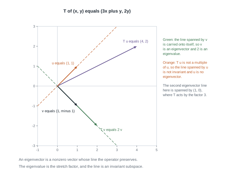
The figure draws that pair: the dashed green line through \((1,-1)\) holds both \(v\) and \(Tv = 2v\), while the dashed orange line through \((1,1)\) misses \(Tu = (4,2)\). So an eigenvector is a nonzero vector whose line the operator preserves, and the object of the week is a preserved subspace rather than a preserved vector.
Three tests for an eigenvalue, and what each one needs
Theorem. Let \(V\) be finite-dimensional over \(F\), let \(T \in \mathcal{L}(V)\), and let \(\lambda \in F\). The following are equivalent: (1) \(\lambda\) is an eigenvalue of \(T\); (2) \(T - \lambda I\) is not injective; (3) \(T - \lambda I\) is not invertible; (4) \(\det(A - \lambda I_n) = 0\) for the matrix \(A = [T]_{\mathcal{B} \leftarrow \mathcal{B}}\) in some, equivalently any, ordered basis \(\mathcal{B}\).
Argument. The first two are a rewriting: \(Tv = \lambda v\) with \(v \ne 0\) says \((T - \lambda I)v = 0\) for some nonzero \(v\), that is, \(\ker(T - \lambda I) \ne \{0\}\), which by Week 3 is failure of injectivity.
For the second and third, \(T - \lambda I\) is an operator on a finite-dimensional space, so rank-nullity applies to it: injectivity makes the nullity zero, forcing the rank up to \(\dim V\) and hence surjectivity, and conversely. So injective, surjective and invertible coincide here. This is where finite-dimensionality is used, and it genuinely fails without it: on \(F^{\mathbb{N}}\), the sequences over \(F\), the right shift \((a_1, a_2, \dots) \mapsto (0, a_1, a_2, \dots)\) is injective and not surjective.
For the third and fourth, fix \(\mathcal{B}\) and set \(A = [T]_{\mathcal{B} \leftarrow \mathcal{B}}\). Week 4 showed \(T \mapsto [T]_{\mathcal{B} \leftarrow \mathcal{B}}\) is a bijection preserving composition and the identity, so \(T - \lambda I\) is invertible exactly when \(A - \lambda I_n\) is. That \(A - \lambda I_n\) is invertible exactly when its determinant is nonzero is the MATH 3312 fact, quoted here and valid over any field. Finally \(\det(\lambda I_n - A) = (-1)^n \det(A - \lambda I_n)\), since negating \(n\) rows scales the determinant by \((-1)^n\), so the two vanish together.
Condition (2) is what proofs want and condition (4) is what a hand computation wants. Note also that the theorem quantifies over \(\lambda \in F\), so enlarging the field can only add eigenvalues.
The characteristic polynomial and the basis it does not remember
Condition (4) asks about one scalar at a time. Making \(\lambda\) a variable packs every eigenvalue into a single object.
Definition. For \(\dim V = n\) finite and \(A = [T]_{\mathcal{B} \leftarrow \mathcal{B}}\), the characteristic polynomial of \(T\) is \(p_T(t) = \det(tI_n - A) \in F[t]\).
Proposition. \(p_T\) is independent of the ordered basis, so the definition is legitimate, and it is monic of degree \(n\).
Argument. Let \(P = P_{\mathcal{C} \leftarrow \mathcal{B}}\) be the invertible change-of-basis matrix of Week 4, so \([T]_{\mathcal{C} \leftarrow \mathcal{C}} = PAP^{-1}\). Since \(P(tI_n)P^{-1} = tI_n\), we get \(tI_n - PAP^{-1} = P(tI_n - A)P^{-1}\), and multiplicativity of the determinant gives \[\det\big(tI_n - PAP^{-1}\big) = \det P \cdot \det(tI_n - A) \cdot \det P^{-1} = \det(tI_n - A),\] because \(\det P \cdot \det P^{-1} = \det(PP^{-1}) = 1\). For the shape, expand as the signed sum over permutations. The identity permutation contributes \(\prod_{i=1}^{n}(t - A_{ii})\), monic of degree \(n\); every other permutation moves at least two indices, so its term omits two diagonal entries and has degree at most \(n - 2\). Nothing cancels the leading \(t^n\).
Three consequences follow. The eigenvalues of \(T\) are exactly the roots of \(p_T\) lying in \(F\); a degree-\(n\) polynomial has at most \(n\) roots in a field, so \(T\) has at most \(\dim V\) distinct eigenvalues; and each coefficient is a similarity invariant, including \(p_T(0) = (-1)^n \det A\) and the coefficient \(-\sum_i A_{ii}\) of \(t^{n-1}\).
One computational fact is used repeatedly below. If \(A\) is upper triangular then so is \(tI_n - A\), whose determinant is the product of its diagonal entries, so \(p_T(t) = \prod_i (t - A_{ii})\): the eigenvalues of a triangular matrix are its diagonal entries, repetitions included. That is why Weeks 13 through 15 chase triangular forms.
Eigenspaces, and how many eigenvalues there can be
Proposition. Let \(T \in \mathcal{L}(V)\) and \(\lambda \in F\), and put \(E_{\lambda} = \ker(T - \lambda I)\). It is a subspace of \(V\); it is nonzero exactly when \(\lambda\) is an eigenvalue; and it is \(T\)-invariant.
Argument. It is the kernel of a linear map, hence a subspace by Week 3, and it is nonzero exactly when \(T - \lambda I\) fails to be injective, which is condition (2). For invariance take \(u \in E_{\lambda}\); then \(Tu = \lambda u \in E_{\lambda}\), since a subspace is closed under scalar multiplication.
Collecting the eigenvectors into one object lets you speak of its dimension. For \(T(x,y) = (3x + y, 2y)\) above, \(E_3 = \operatorname{span}\{(1,0)\}\) and \(E_2 = \operatorname{span}\{(1,-1)\}\) are each one-dimensional and together span \(\mathbb{R}^2\), which is where Week 11 begins.
The dimension of \(E_{\lambda}\) is a separate number from the multiplicity of \(\lambda\) as a root of \(p_T\): the first counts free variables in \((A - \lambda I_n)x = 0\), the second counts factors in a polynomial. The eigenspace dimension is a similarity invariant since \(P^{-1}AP - \lambda I_n = P^{-1}(A - \lambda I_n)P\) forces equal kernel dimensions; the multiplicity is a similarity invariant because \(p_T\) itself does not depend on the ordered basis, by the Proposition above. Week 11 names them the algebraic and geometric multiplicities; this week the honest move is to compute and report both.
Existence is a question about the field
Nothing so far promises that even one eigenvalue exists; the theorem said how to test a candidate, not how to find one. Existence turns on whether \(p_T\) has a root in \(F\) — arithmetic of the field, not size of the space.
An operator on a complex space always has an eigenvalue
Theorem. Let \(F\) be algebraically closed — \(\mathbb{C}\) is the case we use — and let \(V\) be a nonzero finite-dimensional vector space over \(F\). Then every \(T \in \mathcal{L}(V)\) has an eigenvalue in \(F\).
First argument, with determinants. Put \(n = \dim V \ge 1\). Then \(p_T\) is monic of degree \(n \ge 1\), hence not constant, hence has a root \(\lambda \in F\); for \(\mathbb{C}\) this is the fundamental theorem of algebra. Then \(\det(\lambda I_n - A) = 0\), so \(\lambda\) is an eigenvalue.
Second argument, with no determinants at all. Put \(n = \dim V \ge 1\) and pick any \(v \ne 0\). The list \(v, Tv, T^2v, \dots, T^nv\) has \(n+1\) members in an \(n\)-dimensional space, so by Week 2 it is dependent: there are scalars \(a_0, \dots, a_n\), not all zero, with \[a_0 v + a_1 Tv + \dots + a_n T^n v = 0 .\] Let \(m\) be the largest index with \(a_m \ne 0\). Then \(m \ge 1\), since \(m = 0\) would read \(a_0 v = 0\) with \(a_0 \ne 0\) and \(v \ne 0\). Factor \(q(z) = a_0 + a_1 z + \dots + a_m z^m\) over the algebraically closed \(F\) as \(q(z) = a_m(z - \lambda_1)\cdots(z - \lambda_m)\). Substituting \(T\) for \(z\) is legitimate because \(p \mapsto p(T)\) carries sums to sums and products to composites, so \[0 = q(T)v = a_m (T - \lambda_1 I)\cdots(T - \lambda_m I)\,v .\] If every factor \(T - \lambda_j I\) were injective, the composite would be injective, and with \(a_m \ne 0\) the right side could vanish only for \(v = 0\). So some \(T - \lambda_j I\) is not injective, and that \(\lambda_j\) is an eigenvalue.
The second argument is the one to remember. It uses two things only: that \(\dim V\) is finite, so a long enough list is dependent, and that polynomials over \(F\) split into linear factors. No basis, no matrix, no determinant — which is exactly what algebraic closure buys.
The quarter turn, and the fields where an operator stays blind
Example. Let \(R(x,y) = (-y,x)\) be the quarter turn of \(\mathbb{R}^2\), with standard matrix \(\begin{pmatrix} 0 & -1 \\ 1 & 0\end{pmatrix}\), so that \[p_R(t) = \det\begin{pmatrix} t & 1 \\ -1 & t \end{pmatrix} = t^2 + 1,\] which has no real root. So \(R\) has no eigenvalue. Without any determinant: if \(Rv = \lambda v\) with \(v \ne 0\) then \(R^2 v = \lambda^2 v\), and \(R^2 = -I\), so \(\lambda^2 = -1\), which no real scalar satisfies.
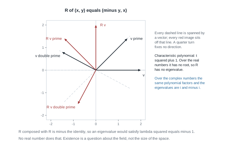
The figure shows what that means geometrically: each dashed line is spanned by a sample vector, each red arrow is its image, and no image lands back on its own line. Since a one-dimensional invariant subspace is an eigenvector line, “no eigenvalue” and “no invariant line” say one thing here. Over \(\mathbb{C}\) the array does not change but the story does: \(t^2 + 1 = (t-i)(t+i)\), and \((1,-i)\) is an eigenvector for \(i\), the matrix sending it to \((i,1) = i\,(1,-i)\).
| Field \(F\) | Operator on \(F^2\) | Characteristic polynomial | Eigenvalues in \(F\) |
|---|---|---|---|
| \(\mathbb{R}\) | \((x,y) \mapsto (-y, x)\) | \(t^2 + 1\) | none |
| \(\mathbb{C}\) | \((x,y) \mapsto (-y, x)\) | \(t^2 + 1\) | \(i\) and \(-i\) |
| \(\mathbb{Q}\) | \((x,y) \mapsto (2y, x)\) | \(t^2 - 2\) | none |
| \(\mathbb{R}\) | \((x,y) \mapsto (2y, x)\) | \(t^2 - 2\) | \(\sqrt{2}\) and \(-\sqrt{2}\) |
| \(\mathbb{F}_2\) | \((x,y) \mapsto (y, x + y)\) | \(t^2 + t + 1\) | none |
The third row is the cheapest failure of all, since \(t^2 - 2\) has no rational root while the identical formula over \(\mathbb{R}\) has two eigenvalues. The last row is checkable by hand: \(\mathbb{F}_2\) holds two scalars, \(t = 0\) gives \(1\) and \(t = 1\) gives \(1 + 1 + 1 = 1\), so that operator has no eigenvalue in a space of four vectors. One positive statement survives over \(\mathbb{R}\): if \(\dim V\) is odd then \(p_T\) has odd degree and so has a real root by the intermediate value theorem. Every real counterexample lives in even dimension.
Invariant subspaces and the block they produce
The quarter turn has no invariant line, but it has invariant subspaces: \(\{0\}\) and \(\mathbb{R}^2\). Widening from preserved lines to preserved subspaces of any dimension is what breaks a hard operator into easier pieces, and every structure theorem ahead works that way.
Definition. A subspace \(U \subseteq V\) is \(T\)-invariant when \(T(U) \subseteq U\). In that case the restriction \(T\vert_U \colon U \to U\), given by \(T\vert_U(u) = Tu\), is an operator on \(U\).
Note what is not being said: not \(T(U) = U\), and not that the vectors of \(U\) stay put. Only that the image of a vector of \(U\) does not escape \(U\) — which is what makes \(T\vert_U\) an operator, so its powers make sense and it has a characteristic polynomial of its own.
Restriction, and the subspaces that are always invariant
Proposition. Let \(T \in \mathcal{L}(V)\) and \(q \in F[t]\). Then \(\ker q(T)\) and \(\operatorname{im} q(T)\) are \(T\)-invariant; in particular so are \(\ker T\), \(\operatorname{im} T\), and every eigenspace \(E_{\lambda} = \ker(T - \lambda I)\).
Argument. What makes it work is that \(T\) commutes with \(q(T)\), a sum of scalar multiples of powers of \(T\). If \(u \in \ker q(T)\) then \(q(T)(Tu) = T\big(q(T)u\big) = 0\), so \(Tu \in \ker q(T)\). If \(w = q(T)v\) then \(Tw = Tq(T)v = q(T)(Tv) \in \operatorname{im} q(T)\). The named cases are \(q(t) = t\) and \(q(t) = t - \lambda\).
The second worked example uses this directly: once \(p_T\) factors, each factor hands you a subspace to look inside. It also settles the relation with eigenvectors, since \(\operatorname{span}\{v\}\) with \(v \ne 0\) is invariant exactly when \(Tv = \lambda v\) for some \(\lambda\). So eigenvectors are precisely the nonzero vectors spanning one-dimensional invariant subspaces.
The adapted basis and the triangular block
Theorem. Let \(\dim V = n\) be finite, \(T \in \mathcal{L}(V)\), and \(U\) a \(T\)-invariant subspace with \(\dim U = k\), \(1 \le k \le n\). Take a basis \((u_1, \dots, u_k)\) of \(U\) and extend it — Week 2 guarantees this — to an ordered basis \(\mathcal{B} = (u_1, \dots, u_n)\) of \(V\). Then \[[T]_{\mathcal{B} \leftarrow \mathcal{B}} = \begin{pmatrix} A & C \\ 0 & D \end{pmatrix},\] where \(A\) is the \(k \times k\) matrix of \(T\vert_U\) in \((u_1, \dots, u_k)\), the zero block is \((n-k) \times k\), and \(C\) and \(D\) are unconstrained.
Argument. Column \(j\) is \([Tu_j]_{\mathcal{B}}\), by the Week 4 definition. For \(j \le k\) we have \(u_j \in U\), so invariance gives \(Tu_j \in U\), so \(Tu_j\) is a combination of \(u_1, \dots, u_k\) alone and its coordinates in slots \(k+1, \dots, n\) vanish. That is the zero block, and the surviving top part of those columns is by definition the matrix of \(T\vert_U\). For \(j > k\) nothing is claimed and nothing is true in general.
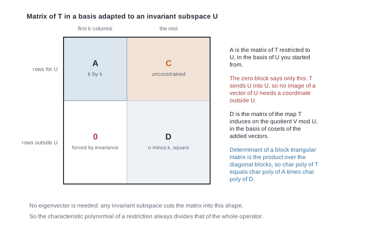
The figure labels the four blocks. Only the lower left is forced, and by one fact — that \(T\) sends \(U\) into \(U\). The upper right is unconstrained, which is why the shape is block upper triangular rather than block diagonal; clearing it too needs an invariant complement, the business of Week 14. The lower right also has a meaning: because \(U\) is invariant, \(\bar{T}(v + U) = Tv + U\) is well defined on the Week 3 quotient \(V/U\), since \(v - v' \in U\) gives \(Tv - Tv' \in U\). The cosets \(u_{k+1} + U, \dots, u_n + U\) are a basis of \(V/U\), and \(D\) is the matrix of \(\bar{T}\).
Corollary. Under the same hypotheses \(p_T(t) = p_{T\vert_U}(t) \cdot p_{\bar{T}}(t)\); in particular the characteristic polynomial of the restriction divides that of \(T\) in \(F[t]\).
Argument. Subtracting \(tI_n\) preserves the shape, giving diagonal blocks \(tI_k - A\) and \(tI_{n-k} - D\), and the MATH 3312 fact about block triangular determinants multiplies them.
The corollary runs both ways: it is how an invariant subspace is exploited once found, and it is how one is hunted, since each factor of \(p_T\) is a place to look. The second worked example does exactly that with a factor having no root in the field.
Worked example — a three by three matrix with a repeated eigenvalue
Work over \(\mathbb{R}\) with \(V = \mathbb{R}^3\), and let \(T\) have matrix \[A = \begin{pmatrix} 4 & -2 & 1 \\ -1 & 3 & 1 \\ 3 & -3 & 2 \end{pmatrix}\] in the standard ordered basis. The task: compute \(p_T\) by hand, factor it, exhibit each eigenspace with a basis, and report the multiplicity of each root beside the dimension of its eigenspace.
Step 1. The characteristic polynomial. Expand \(\det(tI_3 - A)\) along the first row, where \[tI_3 - A = \begin{pmatrix} t-4 & 2 & -1 \\ 1 & t-3 & -1 \\ -3 & 3 & t-2 \end{pmatrix}.\] The three cofactor terms are \[\begin{aligned} (t-4)\big[(t-3)(t-2) + 3\big] &= (t-4)(t^2 - 5t + 9), \\ -2\big[(t-2) - 3\big] &= -2(t-5), \\ (-1)\big[3 + 3(t-3)\big] &= -(3t - 6). \end{aligned}\] Adding, \((t^3 - 9t^2 + 29t - 36) + (-2t + 10) + (-3t + 6) = t^3 - 9t^2 + 24t - 20\).
Step 2. Factor it. Try integer candidates dividing \(20\). At \(t = 2\), \(8 - 36 + 48 - 20 = 0\), so \(t - 2\) divides, and dividing gives \((t-2)(t^2 - 7t + 10) = (t-2)^2(t-5)\). Two checks confirm it: the roots multiply to \(2 \cdot 2 \cdot 5 = 20\), which is \(\det A = 4(6+3) + 2(-2-3) + (3-9) = 36 - 10 - 6 = 20\), and they add to \(9\), the trace \(4 + 3 + 2\).
Step 3. The eigenspace for \(5\). With \[A - 5I_3 = \begin{pmatrix} -1 & -2 & 1 \\ -1 & -2 & 1 \\ 3 & -3 & -3 \end{pmatrix},\] rows one and two coincide and rows one and three are not proportional, so the rank is two and rank-nullity gives \(\dim E_5 = 1\). Row one gives \(z = x + 2y\), row three gives \(z = x - y\); equating, \(3y = 0\), so \(y = 0\) and \(z = x\). Hence \(E_5 = \operatorname{span}\{(1,0,1)\}\), and indeed \(A(1,0,1)^{\mathsf{T}}\) is column one plus column three, \((5,0,5)^{\mathsf{T}} = 5\,(1,0,1)^{\mathsf{T}}\).
Step 4. The eigenspace for \(2\). With \[A - 2I_3 = \begin{pmatrix} 2 & -2 & 1 \\ -1 & 1 & 1 \\ 3 & -3 & 0 \end{pmatrix},\] row three gives \(x = y\), row two then gives \(z = x - y = 0\), and row one is satisfied automatically. So \(E_2 = \operatorname{span}\{(1,1,0)\}\) and \(\dim E_2 = 1\); the rank agrees, since adding twice row two to row one gives \((0,0,3)\) and adding three times row two to row three gives \((0,0,3)\), leaving rank two. Check: \(A(1,1,0)^{\mathsf{T}}\) is column one plus column two, \((2,2,0)^{\mathsf{T}} = 2\,(1,1,0)^{\mathsf{T}}\).
Step 5. Report both numbers separately. The root \(2\) has multiplicity two in \(p_T\) while \(\dim E_2 = 1\); the root \(5\) has multiplicity one and \(\dim E_5 = 1\). The eigenvectors therefore supply only \(1 + 1 = 2 < 3\) dimensions, and no basis of \(\mathbb{R}^3\) consists of eigenvectors of \(T\), since such a basis would have to come from \(E_2 \cup E_5\), which spans a plane. Both multiplicities are similarity invariants, so that is a fact about \(T\) rather than about the array — though \(T\) still has a normal form, which Week 15 supplies. One field remark: every entry and root is an integer, so this reads verbatim over \(\mathbb{Q}\) and \(\mathbb{C}\), while over \(\mathbb{F}_3\) we have \(5 = 2\) and the picture collapses to one eigenvalue.
The same reasoning, transferred
Run the same procedure on a \(2 \times 2\) real matrix whose polynomial refuses to factor. Let \(S\) have standard matrix \[B_0 = \begin{pmatrix} 1 & -2 \\ 1 & 3 \end{pmatrix}, \qquad p_S(t) = \det\begin{pmatrix} t-1 & 2 \\ -1 & t-3\end{pmatrix} = (t-1)(t-3) + 2 = t^2 - 4t + 5 .\] The discriminant is \(16 - 20 = -4\), so there is no real root: \(S\) has no eigenvalue over \(\mathbb{R}\) and preserves no line of \(\mathbb{R}^2\). Over \(\mathbb{C}\) the roots are \(2 \pm i\), a conjugate pair, as they must be for real coefficients. For \(\lambda = 2+i\) the second row of \(B_0 - \lambda I_2\) reads \(x_1 + (1-i)x_2 = 0\), so \(x_2 = 1\) gives \(x_1 = -1+i\). Verify: \(B_0(-1+i, 1)^{\mathsf{T}} = (-3+i,\, 2+i)^{\mathsf{T}}\), and \((2+i)(-1+i) = -2 + 2i - i - 1 = -3+i\). Conjugating gives \((-1-i, 1)\) for \(2-i\).
What stayed the same: the definition, the determinant test, and a polynomial followed by a kernel. What changed: the field, and with it the count, from none to two. The eigenvectors genuinely leave \(\mathbb{R}^2\), since no scalar makes both entries of \((-1+i,1)\) real at once, so the real failure is absence of the object rather than failure to look hard enough.
Second worked example — an invariant plane with no invariant line inside it
Now build an invariant subspace rather than be handed one. Over \(\mathbb{R}\) with \(V = \mathbb{R}^3\), let \(T'\) have standard matrix \[B = \begin{pmatrix} 7 & 6 & 7 \\ 2 & 1 & 1 \\ -6 & -4 & -5 \end{pmatrix}.\]
Step 1. The characteristic polynomial. Expanding \(\det(tI_3 - B)\) along the first row, with \(tI_3 - B = \begin{pmatrix} t-7 & -6 & -7 \\ -2 & t-1 & -1 \\ 6 & 4 & t+5 \end{pmatrix}\), the three terms are \((t-7)(t^2 + 4t - 1)\), whose minor is \((t-1)(t+5) + 4\), then \(6\big[-2(t+5) + 6\big] = 6(-2t-4)\), and then \(-7\big[-8 - 6(t-1)\big] = -7(-6t-2)\). Adding, \((t^3 - 3t^2 - 29t + 7) + (-12t - 24) + (42t + 14) = t^3 - 3t^2 + t - 3\), which groups as \(t^2(t-3) + (t-3) = (t-3)(t^2+1)\). The trace \(7 + 1 - 5 = 3\) matches the \(t^2\) coefficient \(-3\), and \(\det B = 3\) matches the constant term up to sign.
Step 2. The only real eigenvalue. Since \(t^2 + 1\) has no real root, the sole eigenvalue over \(\mathbb{R}\) is \(3\), and solving \((B - 3I_3)x = 0\) gives \(E_3 = \operatorname{span}\{w\}\) with \(w = (2,1,-2)\). Check: \(2(7,2,-6) + (6,1,-4) - 2(7,1,-5) = (6,3,-6) = 3w\).
Step 3. Manufacture the invariant plane. The proposition above makes \(\ker q(T')\) invariant for every \(q\), so take the factor that produced no eigenvector, \(q(t) = t^2 + 1\). Squaring, \[B^2 = \begin{pmatrix} 19 & 20 & 20 \\ 10 & 9 & 10 \\ -20 & -20 & -21 \end{pmatrix}, \qquad B^2 + I_3 = \begin{pmatrix} 20 & 20 & 20 \\ 10 & 10 & 10 \\ -20 & -20 & -20 \end{pmatrix}.\] Check one entry: the \((2,2)\) entry of \(B^2\) is row two against column two, \(2 \cdot 6 + 1 \cdot 1 + 1 \cdot (-4) = 9\), and adding \(1\) gives \(10\). Every row of \(B^2 + I_3\) is a multiple of \((1,1,1)\), so the rank is one and the kernel is the plane \(U = \{(x,y,z) : x + y + z = 0\}\), of dimension two.
Step 4. Restrict and compute. Take \(u_1 = (1,0,-1)\) and \(u_2 = (0,1,-1)\), both on the plane and independent, hence a basis of \(U\): \[Bu_1 = \text{col}_1 - \text{col}_3 = (0,1,-1) = u_2, \qquad Bu_2 = \text{col}_2 - \text{col}_3 = (-1,0,1) = -u_1,\] which confirms invariance directly. Reading off coordinates, \[[T'\vert_U] = \begin{pmatrix} 0 & -1 \\ 1 & 0 \end{pmatrix}, \qquad p_{T'\vert_U}(t) = t^2 + 1 .\] That is the quarter turn again, inside \(\mathbb{R}^3\): the plane is invariant and no line inside it is, since the restriction has no real eigenvalue.
Step 5. Extend and read the block. Add \(u_3 = (1,0,0)\), off the plane since \(1 + 0 + 0 \ne 0\); the matrix with columns \(u_1, u_2, u_3\) has determinant \(1\), so \(\mathcal{B} = (u_1, u_2, u_3)\) is an ordered basis. Now \(Bu_3 = \text{col}_1 = (7,2,-6)\), and writing \(au_1 + bu_2 + cu_3 = (a+c,\, b,\, -a-b)\) gives \(b = 2\), then \(a = 4\), then \(c = 3\). Hence \[[T']_{\mathcal{B} \leftarrow \mathcal{B}} = \begin{pmatrix} 0 & -1 & 4 \\ 1 & 0 & 2 \\ 0 & 0 & 3 \end{pmatrix},\] block upper triangular exactly as the theorem promised. Its characteristic polynomial is \((t-3)(t^2+1)\), matching Step 1 as it must; the restriction’s \(t^2 + 1\) divides \(p_{T'}\) as the corollary requires, and the leftover \(t - 3\) belongs to the induced operator on \(\mathbb{R}^3/U\).
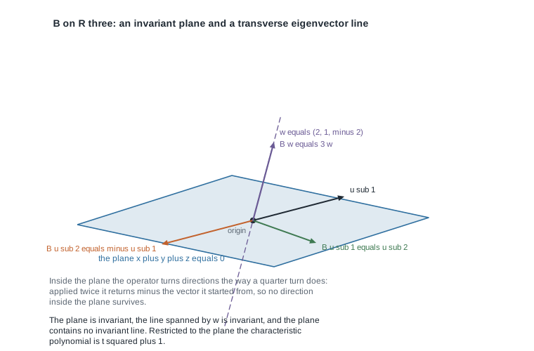
The figure sets the two invariant subspaces side by side. Inside the plane the arrows show \(u_1\), its image \(u_2\), and the image of that, \(-u_1\): applying the operator twice returns the negative of the start, so no direction inside survives. Out of the plane runs the line spanned by \(w = (2,1,-2)\), scaled by \(3\). This operator fails to be diagonalizable over \(\mathbb{R}\) for a reason unlike the first example’s — there the eigenvalues existed and the eigenvectors ran out, here two eigenvalues are not in the field — and it is diagonalizable over \(\mathbb{C}\), where \(3\), \(i\), and \(-i\) are three distinct eigenvalues.
The misreading to avoid
The misreading: every operator has an eigenvalue, so it is only a matter of finding it. This is the habit of a course taught over \(\mathbb{R}\) with examples chosen so the arithmetic works out, and it is false. The quarter turn has characteristic polynomial \(t^2 + 1\) with no real root, and \(R^2 = -I\) leaves no room, since an eigenvalue would satisfy \(\lambda^2 = -1\). True is the theorem with its hypothesis attached — over an algebraically closed field every operator on a nonzero finite-dimensional space has an eigenvalue — plus the consolation that odd real dimension forces one. Keep the quarter turn in your pocket; it returns, disguised, as the invariant plane above.
A neighbouring misreading does more damage in computation: \(\lambda\) is a root of multiplicity \(k\), so \(\dim E_{\lambda} = k\). The first worked example refutes it, with \((t-2)^2\) in \(p_T\) and \(\dim E_2 = 1\). The two numbers report different things — how often a linear factor divides a polynomial, and how many independent vectors solve a homogeneous system — and only one relation holds, which Week 11 proves: the eigenspace dimension is at least one and at most the multiplicity. Confuse them and you declare an operator diagonalizable when it is not.
Two smaller corrections. “The eigenvectors for \(\lambda\) form a subspace” is nearly right: they form \(E_{\lambda}\) with the zero vector added by hand, since \(0\) is excluded from being an eigenvector. And “invariant means \(T\) fixes those vectors” is wrong: invariance says \(T(U) \subseteq U\), and the restriction may move every nonzero vector of \(U\), as the invariant plane does.
Practice on your own
These are for your own checking rather than for submission, and each is within reach of Weeks 1 through 10.
- Both multiplicities on a matrix you build. Produce a \(3 \times 3\) real matrix with characteristic polynomial \((t-2)^2(t-5)\) whose eigenspace for \(2\) has dimension two, verify both by computation, and name a similarity invariant separating it from the first worked example.
- Eigenvalues on a space of polynomials. Let \(D\) be differentiation on \(P_3(\mathbb{R})\), of dimension four. Compute \(p_D\) in the ordered basis \((1, x, x^2, x^3)\), find every eigenvalue and eigenspace, and explain the outcome using \(\ker D\) from Week 3 with no determinant.
- Invariance is not fixing. Let \(U \subseteq \mathbb{R}^3\) be the plane \(x + y + z = 0\). Exhibit two operators leaving \(U\) invariant, one whose restriction has two distinct real eigenvalues and one whose restriction has none, with the characteristic polynomial of each.
- The shift, and where finite-dimensionality entered. On \(F^{\mathbb{N}}\) let \(T\) be the left shift \((a_1, a_2, a_3, \dots) \mapsto (a_2, a_3, \dots)\). Show every \(\lambda \in F\) is an eigenvalue by exhibiting an eigenvector, then say which step of the equivalence theorem breaks for the right shift.
- A field walk. For the operator on \(F^2\) with matrix \(\begin{pmatrix} 0 & 2 \\ 1 & 0\end{pmatrix}\), list the eigenvalues over \(\mathbb{Q}\), \(\mathbb{R}\), \(\mathbb{C}\), and \(\mathbb{F}_2\) — where \(2 = 0\), so compute rather than translate — and say whether an invariant line exists.
Where to read more
- The open lecture notes for MIT OpenCourseWare 18.700 Linear Algebra treat eigenvalues, eigenvectors, and invariant subspaces at this level of abstraction, and are the closest free match to this week.
- MIT OpenCourseWare 18.06 Linear Algebra runs the matrix-first version, with far more numerical characteristic-polynomial practice than this page has room for.
- Treil, Linear Algebra Done Wrong is an openly posted text whose chapter on eigenvalues develops the characteristic polynomial and the field-dependence of existence in an order close to this page’s.
- The optional Roman alignment for this week is the chapter on eigenvalues and eigenvectors, in the sections on eigenvalues and eigenvectors and on invariant subspaces. The textbook is optional for everything on this site — a borrowed or library copy suffices, and nothing here reproduces or adapts it. Availability and licence terms for all sources above are unsettled and are not asserted here.
- Course pages: the notes index, the syllabus, the schedule, and the resources page. The learning management system remains authoritative for section logistics.
Where this goes next
This week produced the raw material and left the organising question open. You can now test a scalar for being an eigenvalue three ways, compute a characteristic polynomial and know it belongs to the operator rather than to an array, exhibit eigenspaces, and turn any invariant subspace into a block upper triangular matrix whose diagonal blocks split that polynomial. Missing is the criterion: when do the eigenvectors reach across the whole space, and what is the best matrix available when they do not?
Week 11, on similar matrices, diagonalization, and multiplicity, takes the first half. It names the algebraic and geometric multiplicities this page reported by hand, proves that eigenvectors for distinct eigenvalues are independent, and gives the exact condition for a basis of eigenvectors: the characteristic polynomial must split over \(F\) and the two multiplicities must agree everywhere. Both worked examples wait on it, the first failing the second condition and the second failing the first over \(\mathbb{R}\) while passing both over \(\mathbb{C}\). Weeks 12 through 15 then push the block triangular shape as far as it goes, ending in the Jordan canonical form. To look back: Week 4 holds the similarity law every computation here used, and the notes index and course home page list what is available.