Week 3 — Uniformly most powerful tests and monotone likelihood ratios
Where this week starts
Week 2 finished with a complete result and an incomplete procedure. The Neyman-Pearson lemma says exactly which test is most powerful when the null and the alternative are both single distributions: threshold the likelihood ratio, randomizing on the boundary if the model is discrete. But the test it hands you was built from one particular alternative \(\theta_1\), and changing \(\theta_1\) changes the critical value and in principle the shape of the rejection region. Real alternatives are rarely single points: a laboratory monitoring a defect rate cares about every rate above the standard.
So this week asks a sharper question: when does one test stay most powerful against every alternative in a set at once? Such a test is called uniformly most powerful, and the word to hold on to is uniformly — the optimality runs over the whole alternative set, and holds within a stated class of competitors, never in the abstract. The property that delivers it is monotone likelihood ratio, the theorem that converts the property into a test is the Karlin-Rubin theorem, and the home of both is the one-parameter exponential family from Week 0.
Two things should feel different by the end. First, “which test is best” is not a well-formed question until you have said best against what and best among which competitors. Second, the two-sided problem should feel like a genuine impossibility rather than an oversight: no cleverer statistic produces a uniformly most powerful test of a normal mean against a two-sided alternative, and the repair narrows the competitors by demanding unbiasedness instead.
Why this matters beyond the theorem
Here is the claim someone gets wrong without this material. An analyst calibrating an instrument runs the one-sided test because a colleague called it the most powerful test available, sees a sample mean well below the reference value, and reports a discrepancy. In the setting worked below that test has power \(0.000134\) at a true mean four units below the reference: it is nearly blind in that direction, and the blindness is not a defect but what it paid for optimality on the other side. Worse, if the direction is chosen after seeing which way the data fell, the procedure’s actual size is \(0.10\) rather than \(0.05\), so the premise that made it optimal has quietly been withdrawn.
The second stake appears in every discrete model, where a test whose stated level is \(0.05\) may have size \(0.032\) because no cutoff lands on the nominal figure. That gap is not free: the conservative test is beaten at every alternative by one that spends the whole allowance.
What you will be able to do
- State what makes a test uniformly most powerful at level \(\alpha\), naming both the alternative set the optimality runs over and the class of competitors it beats.
- Verify or refute monotone likelihood ratio for a stated family in a stated statistic, and give the direction the ratio moves.
- Write a one-parameter exponential family in natural form and read off the sufficient statistic and the sign that fixes that direction.
- Apply the Karlin-Rubin theorem to build the uniformly most powerful one-sided test, including the randomization exact size needs in a discrete model, and derive its power function.
- Show that no uniformly most powerful test exists against a two-sided alternative by exhibiting two level-\(\alpha\) tests neither of which dominates.
- Define an unbiased test, diagnose unbiasedness from a power function, and state the two side conditions identifying the best unbiased test in a one-parameter exponential family.
Terms and notation worth fixing
Three of these are places where loose usage does real damage.
| Symbol or term | Meaning as used in this course |
|---|---|
| \(\Theta_0\), \(\Theta_1\) | the null and alternative parameter sets; this week both are intervals of the real line |
| \(\varphi(x)\) | the test function, the probability of rejecting when the data are \(x\); a non-randomized test takes only the values \(0\) and \(1\) |
| \(\beta(\theta) = E_\theta \varphi(X)\) | the power function, defined on all of \(\Theta\); on \(\Theta_0\) it is the probability of rejecting a true null |
| size and level | the size is \(\sup_{\theta \in \Theta_0} \beta(\theta)\), one number; a level is any \(\alpha\) with size \(\le \alpha\), so a test of size \(0.032\) is a level-\(0.05\) test |
| \(T(X)\) | the statistic the likelihood ratio is monotone in, named every time because the property is relative to it |
| monotone likelihood ratio in \(T\) | for every \(\theta_1 < \theta_2\), the ratio \(f(x; \theta_2)/f(x; \theta_1)\) is a nondecreasing function of \(T(x)\) |
| uniformly most powerful | \(\beta(\theta) \ge \beta_{\psi}(\theta)\) for all \(\theta \in \Theta_1\) and every competitor \(\psi\) in the stated class |
| \(\gamma\) | the probability of rejecting at the one boundary value of \(T\), which buys exact size in a discrete model |
Monotone likelihood ratio as a family property
The Neyman-Pearson region for a simple pair is \(\{x : f(x; \theta_1)/f(x; \theta_0) > k\}\), so whether one test can serve every alternative comes down to a question about that ratio. Does the ordering it puts on the sample space depend on which alternative you picked? Monotone likelihood ratio is the statement that it does not.
The definition and the statistic it names
Let \(\{f(x; \theta) : \theta \in \Theta\}\) be a family of densities or mass functions with \(\Theta \subseteq \mathbb{R}\) an interval, and let \(T\) be a real-valued statistic. The family has monotone likelihood ratio in \(T\) if for every pair \(\theta_1 < \theta_2\) the ratio
\[ \Lambda_{\theta_1, \theta_2}(x) \;=\; \frac{f(x; \theta_2)}{f(x; \theta_1)} \]
is a nondecreasing function of \(T(x)\), on the set where at least one of the two densities is positive, reading the ratio as \(+\infty\) where the denominator vanishes and the numerator does not.
Three features carry the week. It is a property of a pair, a family together with a named statistic, so “this family has monotone likelihood ratio” is an incomplete sentence. Direction is part of the claim: a family whose ratio is nonincreasing in \(T\) has the property in \(-T\), which reflects every region that follows. And the requirement runs over all pairs, which is why it belongs to the family rather than to one testing problem. What it buys is immediate: if \(\Lambda\) is nondecreasing in \(T\) then \(\{x : \Lambda(x) > k\}\) is an upper set of \(T\), so some \(c\) has \(\{T > c\} \subseteq \{\Lambda > k\} \subseteq \{T \ge c\}\), and only the cutoff, never the shape, depends on the alternative.
Why one-parameter exponential families have it
Write the family in natural form, \(f(x; \theta) = h(x) \exp\{\eta(\theta) T(x) - A(\eta(\theta))\}\), with \(\eta\) the natural parameter and \(A\) the cumulant function. For \(\theta_1 < \theta_2\),
\[ \frac{f(x; \theta_2)}{f(x; \theta_1)} \;=\; \exp\bigl\{ [\eta(\theta_2) - \eta(\theta_1)] \, T(x) \bigr\} \cdot \exp\bigl\{ A(\eta(\theta_1)) - A(\eta(\theta_2)) \bigr\} , \]
and the second factor is free of \(x\). So the ratio is strictly increasing in \(T(x)\) exactly when \(\eta(\theta_2) > \eta(\theta_1)\): a one-parameter exponential family whose natural parameter is strictly increasing in \(\theta\) has monotone likelihood ratio in its natural sufficient statistic, and one whose \(\eta\) is strictly decreasing has it in \(-T\). The carrier \(h(x)\) never enters.
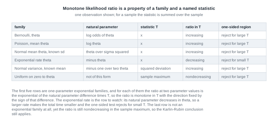
The fourth row of the table is the warning to memorize. For exponential lifetimes with rate \(\theta\) the density is \(\theta e^{-\theta x}\), so \(\eta(\theta) = -\theta\) decreases as the rate grows: the family has the property in \(-\sum_i X_i\), and the one-sided test for a large rate rejects when the total time on test is small. The last row points the other way. The uniform family on \((0, \theta)\) is not an exponential family, its support moving with \(\theta\), yet the ratio \((\theta_1/\theta_2)^n\) below \(\theta_1\), jumping to \(+\infty\) above it, is still nondecreasing in the sample maximum. Exponential structure is sufficient here and necessary for nothing.
A family that fails the property
Let \(X\) be one Cauchy observation with location \(\theta\), density \(f(x; \theta) = \{\pi(1 + (x - \theta)^2)\}^{-1}\). Against \(\theta_1 = 0\) and \(\theta_2 = \theta\) the ratio is
\[ \Lambda(x) \;=\; \frac{1 + x^2}{1 + (x - \theta)^2} , \]
which tends to \(1\) as \(x \to \pm\infty\) and so cannot be monotone unless it is constant. Setting its derivative to zero gives \(x(x - \theta) = 1\), so the maximizer is \(x = \bigl(\theta + \sqrt{\theta^2 + 4}\bigr)/2\). At \(\theta = 2\) that is \(1 + \sqrt{2} \approx 2.414\), where the ratio attains \(\bigl(1 + \sqrt{2}\bigr)^2 \approx 5.828\), while \(\Lambda(10) = 101/65 \approx 1.554\): an observation at \(10\), far out in the direction of the alternative, is weaker evidence for it than one at \(2.4\). Solving \(\Lambda(x) = 5\) gives \(x^2 - 5x + 6 = 0\), so the most powerful region at that cutoff is the bounded interval \((2, 3)\), of null probability \((\arctan 3 - \arctan 2)/\pi = 0.0452\).
That interval is the whole problem. Repeat the construction against \(\theta_2 = 4\) at the same size and the region is \((3.20, 6.16)\), a different set. Since a most powerful test at a given level is essentially unique, no single test is most powerful against both, so no uniformly most powerful test exists even for the one-sided Cauchy problem. Heavy-tailed location families generally fail the property, which is one reason Weeks 12 and 13 build procedures that do not need it.
Karlin-Rubin and the reach of one-sided optimality
Theorem (Karlin-Rubin). Let \(\Theta \subseteq \mathbb{R}\) be an interval, let the family have monotone likelihood ratio in \(T\), and fix \(\theta_0\) in \(\Theta\). For testing \(H_0: \theta \le \theta_0\) against \(H_1: \theta > \theta_0\), define
\[ \varphi(x) = \begin{cases} 1, & T(x) > c, \\ \gamma, & T(x) = c, \\ 0, & T(x) < c, \end{cases} \]
with \(c\) and \(\gamma \in [0, 1]\) chosen so that \(E_{\theta_0} \varphi(X) = \alpha\). Then \(\varphi\) is uniformly most powerful at level \(\alpha\), and its power function \(\beta(\theta) = E_\theta \varphi(X)\) is nondecreasing.
Every hypothesis is used: the parameter must be one-dimensional and ordered, or “one-sided” means nothing, and the property must hold in the same \(T\) for all pairs, since the argument quantifies over alternatives.
Why the power function is nondecreasing
This step is what makes the composite null free. Take \(\theta' < \theta''\) and consider the artificial problem of testing \(\theta'\) against \(\theta''\) at level \(\beta(\theta') = E_{\theta'}\varphi\). By monotone likelihood ratio \(\varphi\) is the Neyman-Pearson test for that pair, hence most powerful at that level. Compare it with the constant test \(\psi \equiv \beta(\theta')\), which ignores the data, has the same level, and has power exactly \(\beta(\theta')\). Most powerful means \(\varphi\) cannot do worse, so \(\beta(\theta'') \ge \beta(\theta')\). Hence the supremum of \(\beta\) over \(\Theta_0 = \{\theta \le \theta_0\}\) is attained at the boundary, and calibrating at the single value \(\theta_0\) makes the test level \(\alpha\) over the whole composite null.
The proof in three moves
Move one, reduce to a simple pair. Fix any \(\theta_1 > \theta_0\). Neyman-Pearson says a most powerful level-\(\alpha\) test of \(\theta_0\) against \(\theta_1\) rejects wherever \(\Lambda(x) = f(x; \theta_1)/f(x; \theta_0) > k\), does not reject wherever \(\Lambda(x) < k\), and may be assigned freely where \(\Lambda(x) = k\) so long as the size comes out right. Choose \(c\) and \(\gamma\) to give size \(\alpha\) at \(\theta_0\) and let \(k\) be the value the ratio takes at \(T = c\). Monotone likelihood ratio then puts \(\varphi\) in exactly that form, since nondecreasing in \(T\) means \(T > c\) forces \(\Lambda \ge k\) and \(T < c\) forces \(\Lambda \le k\), so \(\varphi\) never rejects below the threshold and never withholds rejection above it.
Say why that covers the flat case, because the definition gives only nondecreasing. The ratio may sit at height exactly \(k\) across a whole stretch of values of \(T\) rather than meeting \(k\) at one boundary value, and then \(\{\Lambda > k\}\) is strictly smaller than \(\{T > c\}\): the sharp cut at \(c\) rejects outright at some points of the stretch and not at others. The conclusion survives untouched, because the sufficiency inequality of Week 2 turns on the factor \(f_1 - k f_0\), which vanishes identically there, so the pointwise inequality holds however \(\varphi\) is assigned on the stretch. Where the ratio is strictly increasing in \(T\), as in every exponential family above, the stretch collapses to a single value and the usual picture returns.
Move two, notice what is missing. The pair \((c, \gamma)\) was determined by \(\alpha\) and the null distribution alone. The alternative entered only through the direction of the inequality, which the property fixed once for all pairs, so the same \(\varphi\) is most powerful against every \(\theta_1 > \theta_0\) at once.
Move three, enlarge the null. Every level-\(\alpha\) test for the composite null \(\theta \le \theta_0\) is in particular a level-\(\alpha\) test for the simple null \(\theta = \theta_0\), so the competitors to beat form a subset of the class already handled, and the previous subsection put \(\varphi\) itself in that subset. A rule best in a class and belonging to a subclass is best in the subclass.
Drop the property and move one fails: a most powerful region still exists for each alternative, but its shape depends on which one, as the Cauchy interval showed. Drop one-sidedness and move two fails, since the direction of the inequality is no longer fixed.
Where uniform optimality runs out
Suppose the family has monotone likelihood ratio in \(T\), and test \(H_0: \theta = \theta_0\) against \(H_1: \theta \ne \theta_0\). Against an alternative above \(\theta_0\), move one gives an upper-tail region; against one below, the same argument with the inequality reversed gives a lower-tail region. The necessity half of the Neyman-Pearson lemma pins a most powerful test down only off the tie set where the likelihood ratio equals its threshold, so quote it that way rather than as uniqueness up to probability zero: on a family whose ratio is merely nondecreasing in \(T\) the tie set can carry positive probability. When the ratio is continuously distributed, as it is in the normal model of the second worked example, that tie set is null and the pinning is complete, and then a single test would have to agree almost everywhere with two tests that disagree on a set of positive probability. No uniformly most powerful level-\(\alpha\) test exists, and the second worked example does this with numbers.
Be precise about what failed. Reverse the roles of null and alternative and optimality returns: in a one-parameter exponential family, testing \(H_0: \theta \le \theta_1\) or \(\theta \ge \theta_2\) against \(\theta_1 < \theta < \theta_2\) does have a uniformly most powerful test, rejecting when \(c_1 < T < c_2\). What breaks uniform optimality is a two-sided alternative, asking one region to point two ways at once.
Unbiased tests as the repair
A level-\(\alpha\) test is unbiased when \(\beta(\theta) \le \alpha\) for every \(\theta \in \Theta_0\) and \(\beta(\theta) \ge \alpha\) for every \(\theta \in \Theta_1\): it is never less likely to reject when the null is false than when it is true. That is a coherence demand rather than an optimality criterion, and it is what the one-sided tests fail in a two-sided problem, since the test rejecting for large sample means has power far below \(\alpha\) on the low side.
Two consequences follow when the power function is smooth, as it is in an exponential family, where \(\beta\) may be differentiated under the integral sign in the interior of the natural parameter space. If \(\theta_0\) is a boundary point between \(\Theta_0\) and \(\Theta_1\) and \(\beta\) is continuous, unbiasedness forces \(\beta(\theta_0) = \alpha\), since \(\beta\) is at most \(\alpha\) from one side and at least \(\alpha\) from the other; and if \(\beta\) has an interior minimum at \(\theta_0\) then \(\beta'(\theta_0) = 0\). Those two equalities identify the uniformly most powerful unbiased test in a one-parameter exponential family against a two-sided alternative: it rejects when \(T \le c_1\) or \(T \ge c_2\), with the constants fixed by
\[ E_{\theta_0} \varphi(X) = \alpha \qquad \text{and} \qquad E_{\theta_0}\bigl[ T(X)\, \varphi(X) \bigr] = \alpha \, E_{\theta_0} T(X) , \]
the second being \(\beta'(\theta_0) = 0\) written out, since differentiating \(\beta\) with respect to the natural parameter gives \(E_{\theta_0}[T\varphi] - A'(\eta_0) E_{\theta_0}[\varphi]\). For a normal mean with known variance, symmetry of the null distribution makes the familiar equal-tailed test satisfy both at once. Do not generalize that shortcut: for the normal variance with known mean, equal tails fail the second condition.
Worked example — the one-sided binomial test at level 0.05
The model and the question. A quality audit inspects \(n = 20\) items independently, each defective with probability \(\theta\). The process standard is a defect rate of \(0.2\) and the audit exists to detect deterioration, so test \(H_0: \theta \le 0.2\) against \(H_1: \theta > 0.2\) at level \(0.05\).
Step 1: exponential family form. Writing the Bernoulli mass function as \(f(x; \theta) = (1 - \theta)\exp\{x \log[\theta/(1 - \theta)]\}\) for \(x \in \{0, 1\}\) identifies the natural parameter \(\eta(\theta) = \log[\theta/(1-\theta)]\), the log odds, strictly increasing on \((0, 1)\). The natural sufficient statistic is \(T = \sum_{i=1}^{20} X_i\), with \(T \sim \text{Binomial}(20, \theta)\).
Step 2: verify the property in that statistic. For \(\theta_1 < \theta_2\) the ratio of the mass functions of \(T\) is
\[ \frac{f(t; \theta_2)}{f(t; \theta_1)} \;=\; \left( \frac{1 - \theta_2}{1 - \theta_1} \right)^{\!20} \left( \frac{\theta_2 (1 - \theta_1)}{\theta_1 (1 - \theta_2)} \right)^{\!t} , \]
the binomial coefficient having cancelled. The bracket in the second factor is an odds ratio and exceeds \(1\) whenever \(\theta_2 > \theta_1\), so the ratio is strictly increasing in \(t\). With \(\theta_1 = 0.2\) and \(\theta_2 = 0.4\) it is \((0.4 \times 0.8)/(0.2 \times 0.6) = 8/3 \approx 2.667\), so the log ratio is a straight line in \(t\) of slope \(\log(8/3) = 0.981\).
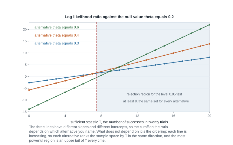
The figure is move one drawn: three alternatives give three lines with three cutoffs, and because all three increase, all three name an upper tail of \(T\).
Step 3: apply the theorem and find the cutoff. The parameter space \((0, 1)\) is an interval, \(\theta_0 = 0.2\) lies inside it, and the property holds in \(T\), so the uniformly most powerful level-\(0.05\) test rejects for large \(T\) with randomization at one boundary value. Under \(\theta_0 = 0.2\) the exact tails are \(P(T \ge 8) = 0.03214\) and \(P(T \ge 7) = 0.08669\), so no non-randomized upper-tail region has size \(0.05\). In the notation of the theorem take \(c = 7\): reject outright when \(T > 7\), and reject with probability \(\gamma\) when \(T = 7\), where
\[ \gamma \;=\; \frac{0.05 - P_{0.2}(T \ge 8)}{P_{0.2}(T = 7)} \;=\; \frac{0.05 - 0.03214}{0.05455} \;=\; 0.3274 . \]
Step 4: the power function. By construction \(\beta(\theta) = P_\theta(T \ge 8) + 0.3274 \, P_\theta(T = 7)\), which is \(0.0500\) at \(\theta = 0.2\) and \(0.2815\), \(0.6384\), \(0.8926\) at \(\theta = 0.3\), \(0.4\), \(0.5\). Dropping the randomization leaves a test of size \(0.03214\) whose power at \(0.4\) is \(0.5841\).
n <- 20; theta0 <- 0.2; alpha <- 0.05
cstar  <- qbinom(1 - alpha, n, theta0) + 1               # 8
p_tail <- 1 - pbinom(cstar - 1, n, theta0)               # 0.032143
gam    <- (alpha - p_tail) / dbinom(cstar - 1, n, theta0) # 0.327358
power <- function(th) 1 - pbinom(cstar - 1, n, th) + gam * dbinom(cstar - 1, n, th)
power(c(0.2, 0.3, 0.4, 0.5))       # 0.0500 0.2815 0.6384 0.8926
1 - pbinom(cstar - 1, n, 0.4)      # 0.5841, the conservative test

lr <- dbinom(0:20, n, 0.4) / dbinom(0:20, n, theta0)
all(diff(lr) > 0)                  # TRUE: the ratio increases in the count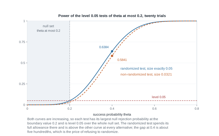
What this licenses and what it does not. Both curves rise, which is the monotonicity proved above, so each test has its largest null rejection probability at \(\theta = 0.2\) and is genuinely level \(0.05\) over all of \(\theta \le 0.2\); at \(\theta = 0.1\) the randomized test rejects with probability \(0.00106\). That test is uniformly most powerful among level-\(0.05\) tests of this one-sided pair, and the figure shows it above the conservative test everywhere. The claim dies as soon as the setup moves: it says nothing about an audit that would also act on an unexpectedly low rate. And the conservative test most laboratories would actually run is uniformly most powerful at level \(0.032\), not at \(0.05\) — a weaker claim, bought by refusing to let a random number settle a borderline case.
The same reasoning, transferred
Now put \(n = 12\) components on a burn-in rack with independent exponential lifetimes of rate \(\theta\) per hour, and test \(H_0: \theta \le 0.5\) against \(H_1: \theta > 0.5\) at level \(0.05\). The natural parameter \(\eta(\theta) = -\theta\) is strictly decreasing, so the family has the property in \(-\sum_i X_i\) and Karlin-Rubin rejects for small total time on test. The exact null distribution is available because \(2\theta \sum_i X_i \sim \chi^2_{24}\), so with the chi-square \(0.05\) quantile at twenty-four degrees of freedom equal to \(13.848\) the test rejects when \(\sum_i X_i \le 13.848\) hours, that is when the mean lifetime is at most \(1.154\) hours. Its power is \(\beta(\theta) = P\bigl(\chi^2_{24} \le 27.696\,\theta\bigr)\), which returns \(0.05\) at \(\theta = 0.5\) and \(0.727\) at \(\theta = 1\).
What stayed the same: an exponential family, a sufficient statistic, the property verified in that statistic, and a size attained at the boundary. What changed: the natural parameter decreases in \(\theta\), so the region is a lower tail, and the statistic is continuous, so the cutoff sits exactly at level \(0.05\). Discreteness belongs to the binomial model, not to the theorem.
Second worked example — the two-sided normal mean with no best test
The model and the question. An instrument is checked against a reference material whose stated value is \(100\). Twenty-five independent measurements are modelled as \(N(\theta, \sigma^2)\) with \(\sigma = 10\) known from calibration history, so \(\bar{X} \sim N(\theta, 4)\) with standard error \(2\). Test \(H_0: \theta = 100\) against \(H_1: \theta \ne 100\) at level \(0.05\); miscalibration either way matters, which makes the alternative two-sided.
Step 1: two one-sided competitors. Let \(\varphi_+\) reject when \(\bar{X} \ge 100 + 1.645 \times 2 = 103.290\) and \(\varphi_-\) reject when \(\bar{X} \le 96.710\). Each has size exactly \(0.05\), so each is a level-\(0.05\) test of this problem, and each is uniformly most powerful for its own one-sided alternative, the normal family with known variance having monotone likelihood ratio in \(\bar{X}\).
Step 2: compare their power. At \(\theta = 104\),
\[ \beta_+(104) = 1 - \Phi\!\left( \frac{103.290 - 104}{2} \right) = 1 - \Phi(-0.355) = 0.6388 , \qquad \beta_-(104) = \Phi\!\left( \frac{96.710 - 104}{2} \right) = 0.0001 . \]
By symmetry the two exchange at \(\theta = 96\), where \(\beta_-(96) = 0.6388\) and \(\beta_+(96) = 0.000134\).
Step 3: the equal-tailed test. It rejects when \(|\bar{X} - 100| \ge 1.96 \times 2 = 3.920\), that is when \(\bar{X} \le 96.080\) or \(\bar{X} \ge 103.920\). Its power at \(104\) is \(\Phi(-3.960) + 1 - \Phi(-0.040) = 0.5160\), and the same at \(96\).
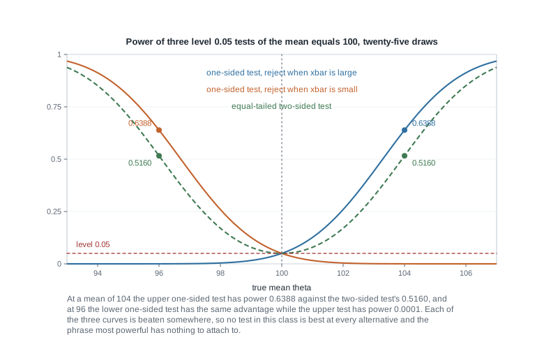
Step 4: no uniformly most powerful test exists. Suppose some level-\(0.05\) test \(\varphi^*\) were one. At \(\theta = 104\) it would need \(\beta^*(104) \ge 0.6388\); but \(\varphi_+\) is the most powerful level-\(0.05\) test of \(100\) against \(104\), and by the necessity half of the Neyman-Pearson lemma any test attaining that power agrees with \(\varphi_+\) almost everywhere off the tie set where the likelihood ratio equals its threshold. Here the ratio is a strictly increasing function of the continuously distributed \(\bar{X}\), so the tie set is the single point \(\bar{X} = 103.290\) and has probability zero, leaving \(\varphi^* = \varphi_+\) almost everywhere. The same argument at \(\theta = 96\) forces \(\varphi^* = \varphi_-\) almost everywhere. The two differ on \(\{\bar{X} \ge 103.290\}\), an event of null probability \(0.05\), so no such \(\varphi^*\) exists. The figure draws the same fact: every curve is beaten somewhere.
Step 5: the repair and its price. Since \(\beta_+(96) = 0.000134\) sits far below \(0.05\) at an alternative, \(\varphi_+\) is not unbiased here, and restricting to unbiased tests eliminates both one-sided tests at once. The equal-tailed test meets the two side conditions, its size being \(0.05\) and its power function having a stationary minimum at \(100\) by symmetry, so it is uniformly most powerful unbiased. Its power of \(0.5160\) at \(\theta = 104\) against \(0.6388\) is what the insurance cost.
se    <- 10 / sqrt(25)                       # 2
cut_u <- 100 + qnorm(0.95) * se              # 103.2897
cut_2 <- 100 + qnorm(0.975) * se             # 103.9199
b_up  <- function(th) 1 - pnorm(cut_u, th, se)
b_two <- function(th) pnorm(200 - cut_2, th, se) + 1 - pnorm(cut_2, th, se)
c(b_up(104), b_two(104))                     # 0.6388 0.5160
c(b_up(96),  b_two(96))                      # 0.0001 0.5160
Size \(0.05\) alone does not deliver unbiasedness. Split the tails unequally, rejecting when \(\bar{X} \ge 100 + 2.3263 \times 2 = 104.653\) or \(\bar{X} \le 100 - 1.7507 \times 2 = 96.499\), and the size is still \(0.01 + 0.04 = 0.05\). That power function is least where the normal densities at the two cutoffs balance, at the midpoint \(\theta = 100.576\), where it takes the value \(0.0415\).
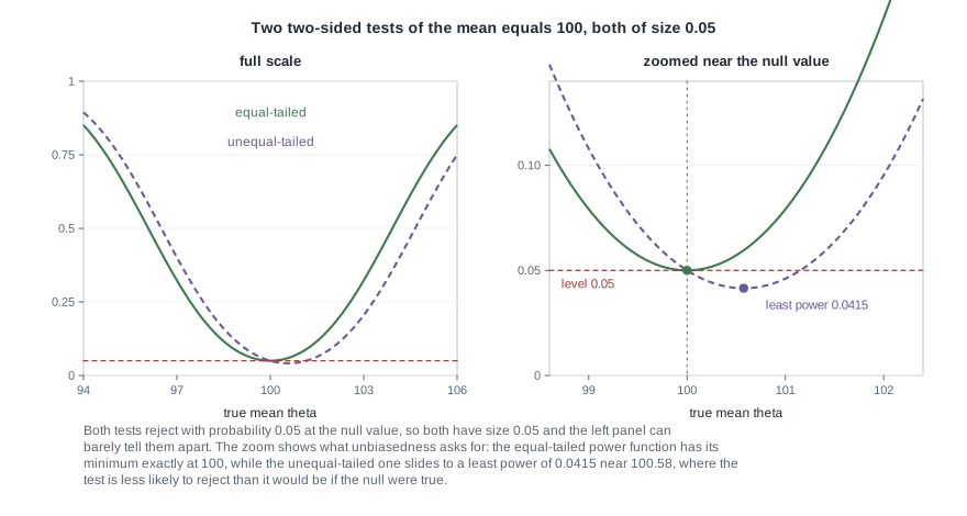
What this licenses and what it does not. At a true mean of \(100.576\) the unequal-tailed test rejects less often than if the null were exactly true, which is bias, and is why the class had to be narrowed by a condition rather than by taste. What it does not license is calling the equal-tailed test best in any wider sense: it is best among unbiased tests, and beaten by a one-sided test on either side.
The misreading to avoid
The misreading sounds like this: “The one-sided test is the most powerful test at level \(0.05\), so I should use it and stop giving power away to the two-sided test.” Two things are wrong, and only the second is arithmetic. First, “most powerful” is not a property a test carries on its own; it is a relation to an alternative set and a class of competitors. The one-sided test above is uniformly most powerful against \(\theta > 100\) among level-\(0.05\) tests, and against \(\theta < 100\) it has power \(0.000134\) at a mean of \(96\), worse than ignoring the data and rejecting with probability \(0.05\). Second, the power it seems to give away is bought with a commitment made before the data. Choose the direction after seeing which way the sample mean fell and you are running the union of two size-\(0.05\) regions, a procedure of size \(0.10\), so the premise that made it optimal is gone.
A second misreading travels with it: “this family has monotone likelihood ratio, so the test rejects for large values of the statistic.” The property relates a family to a named statistic, and its direction is part of the claim. The exponential rate row of the table figure is the trap: since \(\eta(\theta) = -\theta\), the family has the property in minus the total time on test, and the test for a large rate rejects when that total is small.
The third is the reflex that “no uniformly most powerful test exists” means nothing is optimal, so any reasonable test will do. Optimality did not disappear; it changed classes. Narrow the competitors to unbiased tests and a best test returns, pinned down by the two side conditions; change the criterion to average or worst-case risk and best rules return in the forms Week 14 develops. Nonexistence of a uniform optimum says only that a partial ordering has no greatest element, the fact Week 1 met when two risk curves crossed.
Practice on your own
These are for self-checking as you read, not for submission. Work each with a pencil before touching R.
- Verify the property, then break it. For \(X_1, \dots, X_n\) independent \(N(\theta, \sigma^2)\) with \(\sigma^2\) known, write the likelihood ratio at \(\theta_1 < \theta_2\), confirm it increases in \(\bar{X}\), and state the uniformly most powerful test of \(H_0: \theta \le \theta_0\). Then for \(N(\theta, \theta^2)\) with \(\theta > 0\) show the ratio involves both \(\sum_i X_i\) and \(\sum_i X_i^2\), in a combination that changes with the pair, so neither alone can serve as \(T\).
- A family outside the exponential class. For \(X_1, \dots, X_n\) uniform on \((0, \theta)\), show the ratio is nondecreasing in \(X_{(n)}\), derive the uniformly most powerful level-\(\alpha\) test of \(H_0: \theta \le \theta_0\), and check that its cutoff is \(\theta_0 (1 - \alpha)^{1/n}\). Say which Week 0 regularity conditions this never needed.
- The discrete cutoff again. For \(n = 10\) independent Poisson counts with mean \(\theta\), test \(H_0: \theta \le 2\) against \(H_1: \theta > 2\) at level \(0.05\): find the smallest non-randomized upper-tail region and its exact size, compute the randomization probability that restores exact size, and compare both power functions at \(\theta = 3\).
- The Cauchy interval. Confirm the maximizer \(\bigl(\theta + \sqrt{\theta^2 + 4}\bigr)/2\), that the region where the ratio exceeds \(5\) is \((2, 3)\) when \(\theta = 2\), and that it has null probability \(0.0452\). Then say why a bounded region that moves with the alternative rules out uniform optimality.
- A simulation that shows the crossing. Simulate the two-sided normal problem at \(n = 25\) and \(\sigma = 10\) across true means from \(94\) to \(106\), estimate the power of \(\varphi_+\), \(\varphi_-\), and the equal-tailed test at each, and plot the three curves with Monte Carlo standard errors.
Where to read more
- MIT OpenCourseWare 18.655 Mathematical Statistics treats uniformly most powerful testing and monotone likelihood ratio in its hypothesis-testing lectures.
- Penn State STAT 415 Introduction to Mathematical Statistics is the gentler open reference, and the place to rebuild Week 2 if the proof above moved too fast.
- The optional Hogg, McKean, and Craig alignment for this week is Chapter 8.2, which develops uniformly most powerful tests and monotone likelihood ratio in the order used here. The text is optional throughout this course and is never required to be purchased; availability and licence terms for every source listed here are still being confirmed.
- Computing runs on The R Project for Statistical Computing and Quarto; nothing above needs more than the
statspackage that ships with R. - The course pages: the syllabus, the schedule, the resources overview, and the notes index.
Where this goes next
Week 4 turns every test on this page into an interval. The device is duality: a family of level-\(\alpha\) acceptance regions, one for each candidate parameter value, becomes a \(1 - \alpha\) confidence set by collecting the values whose region contains the observed data. The one-sided test built here inverts into a one-sided bound and the two-sided test into the familiar interval, so this week’s power question reappears as a question about what an interval is asked to say. The discreteness that forced a randomization probability of \(0.3274\) reappears too, as the conservatism of an exact interval for a proportion.
Read Week 4 — Confidence-test duality, pivots, and exact procedures next, and return to the notes index for the full sequence. If move one felt like a quotation rather than a step you could reproduce, reread Week 2 — Tests as decision rules and the Neyman-Pearson lemma first: every optimality claim from here to Week 6 is built on it.