Week 0 — Readiness review from Mathematical Statistics I
Where this week starts
This page reviews; it does not establish. Every idea below was built in Mathematical Statistics I, and the fifteen weeks that follow treat all of it as available equipment. What is new here is the arrangement. You are about to spend a semester asking what a procedure decides, under what conditions it may decide it, and how badly it behaves when those conditions are strained, and that question keeps reaching back for the same six tools: likelihood and information, sufficiency and exponential families, the limit theorems that license every large-sample approximation, loss and risk, the geometry of projections and quadratic forms, and a simulation habit disciplined enough that a calibration claim can be checked rather than asserted.
Read this page with a pencil and a running self-diagnosis. A student arriving from a different first course usually finds four or five of the six strands comfortable and one or two thin, and the thin ones are rarely the same for any two students. If a strand here reads as unfamiliar rather than merely rusty, work the corresponding bridge material during the first two weeks of the term, rather than discovering the gap in Week 5 when three test statistics are being read off one log-likelihood curve at once.
What Mathematical Statistics I mostly left unfinished is the second half of every sentence. You learned that the maximum likelihood estimator is consistent and asymptotically normal under regularity conditions. This course keeps asking which regularity, why that condition and not another, what breaks first when it fails, and how far the failure propagates into a reported interval or error rate. So this review puts the conditions in front rather than in a footnote, and sets at least one explicit failure beside each result.
Why this matters beyond the theorem
Consider a reliability laboratory that tests forty components, fits an exponential failure model, and reports a symmetric interval for the failure rate built from the normal approximation. Three things have quietly been assumed: that the estimator is roughly unbiased at this sample size, that its sampling distribution is roughly symmetric, and that replacing the unknown information by its estimate costs nothing. In this model at this sample size the first is wrong by about two and a half percent of the estimate, and the second is wrong in a direction that pushes both ends of the interval the same way. The interval is not worthless, but it is not what it claims either, and the exact interval sits noticeably to its right.
That gap between what a procedure claims and what it delivers is the subject of the whole course: a level-\(\alpha\) test whose actual size is not \(\alpha\), a nominal ninety-five percent interval whose coverage is ninety-one percent, a chi-square approximation used where the limit theorem does not apply. Diagnosing any of those means comparing an approximation against something exact, and the exact object is usually a likelihood, a projection, or a risk function.
What you will be able to do
- Write the log-likelihood for a one-parameter model, derive the score and the Fisher information, solve for the maximum likelihood estimator, and state the regularity conditions that make the normal approximation legitimate.
- Verify sufficiency by the factorization criterion, put a family in one-parameter exponential form, and read the mean and variance of the natural sufficient statistic off the cumulant function.
- Distinguish convergence in probability from convergence in distribution, and apply Slutsky’s theorem and the delta method with their conditions stated rather than assumed.
- Compare risk functions under squared-error loss, decompose mean squared error into variance and squared bias, and derive an elementary Bayes estimator as a posterior expectation.
- Diagnose a linear model computation as a projection: identify the model subspace, verify that the hat matrix is symmetric and idempotent, and read degrees of freedom as a rank rather than a count of parameters.
- Run a simulation study that estimates bias, variance, and mean squared error, and report its Monte Carlo uncertainty separately from the statistical uncertainty it measures.
Terms and notation worth fixing
The whole course uses one notation, and it is worth spending a minute now so that no later derivation stalls on a symbol. These are the conventions in force from here on.
| Symbol or term | Meaning as used in this course |
|---|---|
| \(\theta\), \(\Theta\) | the parameter and the parameter space; \(\Theta_0\) and \(\Theta_1\) arrive in Week 2 as null and alternative sets |
| \(\ell(\theta)\) | the log-likelihood for the observed sample, a function of \(\theta\) with the data held fixed |
| \(U(\theta)\) | the score, \(\partial \ell(\theta) / \partial \theta\); maximum likelihood sets it to zero |
| \(I_1(\theta)\), \(I_n(\theta)\) | Fisher information from one observation and from the sample; for independent identically distributed data \(I_n(\theta) = n I_1(\theta)\) |
| \(\hat\theta\) | the maximum likelihood estimator, a random variable until the data are realized |
| \(L(\theta, a)\), \(R(\theta, \delta)\) | the loss of action \(a\) when the state is \(\theta\), and the risk \(R(\theta, \delta) = E_\theta L(\theta, \delta(X))\) of the procedure \(\delta\) |
| \(T(X)\) | a statistic, usually the sufficient statistic of the model under discussion |
| \(H\) | the hat matrix \(X(X^{\top}X)^{-1}X^{\top}\), the orthogonal projection onto the column space of the design matrix |
The likelihood object and what it carries
Fix a family of densities or mass functions \(f(x; \theta)\) indexed by \(\theta \in \Theta\), and observe \(x = (x_1, \dots, x_n)\). The likelihood \(\mathcal{L}(\theta) = f(x; \theta)\) is that same function read backwards: the data are frozen and \(\theta\) varies. That reversal is where the most common misunderstanding of the term begins. The likelihood is not a probability distribution over \(\theta\): it does not integrate to one over \(\Theta\), and two likelihoods differing by a positive constant free of \(\theta\) carry identical information. Only ratios and derivatives in \(\theta\) are meaningful, which is why the log-likelihood \(\ell(\theta) = \log \mathcal{L}(\theta)\), whose differences are log ratios, is the object everything is built from.
Almost every asymptotic result in this course requires the same short list of conditions, so state them once here and refer back. The family must be identifiable, so that distinct parameter values give distinct distributions. The support \(\{x : f(x; \theta) > 0\}\) must not depend on \(\theta\). The true \(\theta\) must lie in the interior of \(\Theta\), not on its boundary. The map \(\theta \mapsto f(x; \theta)\) must be twice continuously differentiable near the true value, and differentiation under the integral sign must be valid there, which is what allows an interchange of \(\partial / \partial \theta\) with \(\int \cdot \, dx\). And the information must be finite and strictly positive. A seventh condition is what the asymptotic normality of the maximum likelihood estimator specifically needs, and it is the one most often left silent: the third derivative \(\partial^3 \log f(x; \theta) / \partial \theta^3\) must exist near the true value and be bounded there by a function \(M(x)\) with \(E_\theta M(X) < \infty\), which controls the remainder when the score is expanded about the true value. Every one of these is violated by some standard model, and each violation breaks a different link in the chain.
Score, information, and the two identities
The score is \(U(\theta) = \partial \ell(\theta) / \partial \theta\), the local slope of the log-likelihood. Two identities do most of the work all semester. Both come from differentiating the statement that a density integrates to one.
\[ \int f(x; \theta) \, dx = 1 \quad \Longrightarrow \quad \int \frac{\partial}{\partial \theta} f(x; \theta) \, dx = 0 \quad \Longrightarrow \quad E_\theta \left[ \frac{\partial}{\partial \theta} \log f(X; \theta) \right] = 0 . \]
The last step multiplies and divides by \(f(x; \theta)\), which is legitimate on the support, and the support does not move with \(\theta\). So the score has mean zero, and its variance defines the Fisher information. Writing \(U_1(\theta)\) for the score contributed by a single observation, \(I_1(\theta) = \operatorname{Var}_\theta U_1(\theta) = E_\theta[U_1(\theta)^2]\), the second equality holding because the mean is zero. Differentiating once more and interchanging again gives the second identity,
\[ I_1(\theta) \;=\; E_\theta\!\left[ \left( \frac{\partial}{\partial \theta} \log f(X; \theta) \right)^{\!2} \right] \;=\; - E_\theta\!\left[ \frac{\partial^2}{\partial \theta^2} \log f(X; \theta) \right] , \]
which says that information is expected curvature. A sharply peaked log-likelihood is an informative one. The first identity used the interchange once and the second used it twice, and both fail when the support depends on the parameter. The standard counterexample is worth carrying in your head: for \(X_1, \dots, X_n\) uniform on \((0, \theta)\), the likelihood is \(\theta^{-n}\) for \(\theta \ge \max_i x_i\) and zero below it, so it is not differentiable at the maximizer. Be exact about what fails there. The score is not missing: on the support \(\ell(\theta) = -n \log \theta\), so \(U(\theta) = -n/\theta\) exists at every \(\theta\) above the sample maximum. The mean-zero identity is therefore not meaningless but false, since \(E_\theta U(\theta) = -n/\theta \ne 0\), which is exactly the computation Practice item 2 asks you to carry out directly. The invalid step is the interchange, and it is invalid because the support moves with \(\theta\). The maximum likelihood estimator is \(X_{(n)}\), the sample maximum, and it converges at rate \(n\) rather than \(\sqrt{n}\): since \(P_\theta(n(\theta - X_{(n)})/\theta > t) = (1 - t/n)^n \to e^{-t}\), the limit law is exponential, not normal. Nothing about the usual theory survives, and the reason is the one condition that was dropped.
Sufficiency, factorization, and exponential families
A statistic \(T(X)\) is sufficient for \(\theta\) when the conditional distribution of \(X\) given \(T(X) = t\) does not depend on \(\theta\). The workable criterion is the factorization theorem: for a family dominated by a common \(\sigma\)-finite measure, \(T\) is sufficient if and only if \(f(x; \theta) = g(T(x); \theta) \, h(x)\) for some non-negative \(g\) and \(h\). In practice you write the joint density and look for the parameter to travel only in company with a single function of the data.
The one-parameter exponential family is where that pattern is structural rather than lucky. Write \(f(x; \theta) = h(x) \exp\{\eta(\theta) T(x) - A(\eta(\theta))\}\), with \(\eta\) the natural parameter and \(A\) the cumulant function. Factorization is immediate, so \(\sum_i T(x_i)\) is sufficient for a sample. In the natural parameterization the cumulant function does double duty: \(A'(\eta) = E_\eta T(X)\) and \(A''(\eta) = \operatorname{Var}_\eta T(X)\), so moments come from differentiation rather than integration. When the natural parameter space contains an open set the family is also complete, and completeness plus sufficiency upgrades the Rao-Blackwell improvement into the Lehmann-Scheffé uniqueness statement. Keep the direction of Rao-Blackwell exact, since Week 14 reuses it: conditioning any estimator on a sufficient statistic cannot increase risk under a convex loss, by Jensen’s inequality applied conditionally. And sufficiency is always relative to a model. A statistic sufficient under the exponential model carries no such guarantee under a Weibull model, so “we lost nothing by reducing the data” is a claim about the model, never about the data.
Limits that license the approximations
Two convergence notions are in play and they are not interchangeable. \(X_n \to_p X\) means \(P(|X_n - X| > \epsilon) \to 0\) for every \(\epsilon > 0\): the random variables get close to each other. \(X_n \to_d X\) means \(F_n(x) \to F(x)\) at every continuity point of \(F\): the distributions get close, and the random variables need not live on the same space at all. Convergence in probability implies convergence in distribution; the converse fails except when the limit is a constant, in which case the two coincide. The weak law of large numbers delivers the first kind for sample means, the central limit theorem delivers the second kind for standardized sample means, and the continuous mapping theorem transports both through any function whose discontinuities carry probability zero under the limit law.
That last transport is used more often than it is named. In the exponential model below, \(\bar{X} \to_p 1/\theta\) by the weak law, and the map \(u \mapsto 1/u\) is applied at the point \(u = 1/\theta\), not at \(\theta\); its only discontinuity sits at \(u = 0\), so continuity at the point of evaluation asks that the mean lifetime \(1/\theta\) stay away from zero, and \(\hat\theta = 1/\bar{X} \to_p \theta\) follows. Get the dangerous direction right: it is \(\theta \to \infty\), where \(1/\theta\) approaches the discontinuity. As \(\theta \downarrow 0\) the mean lifetime runs off to infinity instead, and the map is perfectly well behaved there.
Slutsky’s theorem and where the constant matters
Slutsky’s theorem states that if \(X_n \to_d X\) and \(Y_n \to_p c\) for a constant \(c\), then \(X_n + Y_n \to_d X + c\), \(X_n Y_n \to_d cX\), and, provided \(c \neq 0\), \(X_n / Y_n \to_d X / c\). The constancy of \(c\) is not a technicality that a careful proof could remove. Take \(X_n\) standard normal for every \(n\) and set \(Y_n = -X_n\). Then \(X_n \to_d N(0, 1)\) and \(Y_n \to_d N(0, 1)\) as well, yet \(X_n + Y_n = 0\) for every \(n\), which is nowhere near the \(N(0, 2)\) that adding the two limit laws would suggest. Marginal convergence in distribution says nothing about joint behaviour; what rescues the argument is that \(Y_n \to_p c\) with \(c\) constant forces the pair \((X_n, Y_n)\) to converge jointly to \((X, c)\), which is exactly what marginal convergence alone never gives.
The standard use is studentization. If \(\sqrt{n}(\hat\theta - \theta) \to_d N(0, v(\theta))\) with \(v(\theta) > 0\), and \(\hat{v}\) is any consistent estimator of it, write the studentized quantity as a product,
\[ \frac{\sqrt{n}(\hat\theta - \theta)}{\sqrt{\hat{v}}} \;=\; \frac{\sqrt{n}(\hat\theta - \theta)}{\sqrt{v(\theta)}} \cdot \sqrt{\frac{v(\theta)}{\hat{v}}} , \]
where the first factor converges in distribution to a standard normal and the second converges in probability to one. Slutsky then gives a standard normal limit for the ratio. Every Wald interval you have ever computed is this line, and this is also where Week 5 will begin.
The delta method and where it breaks
If \(\sqrt{n}(\hat\theta - \theta) \to_d N(0, v(\theta))\) and \(g\) is differentiable at \(\theta\) with \(g'(\theta) \neq 0\), then
\[ \sqrt{n}\,\bigl(g(\hat\theta) - g(\theta)\bigr) \to_d N\bigl(0, \; g'(\theta)^2 \, v(\theta)\bigr) . \]
The proof is one expansion and one appeal to Slutsky. The quickest sketch uses the mean value theorem, \(g(\hat\theta) - g(\theta) = g'(\tilde\theta)(\hat\theta - \theta)\) for some \(\tilde\theta\) between \(\hat\theta\) and \(\theta\), with \(\tilde\theta \to_p \theta\) and hence \(g'(\tilde\theta) \to_p g'(\theta)\); note that this sketch quietly asks for \(g'\) to exist near \(\theta\) and be continuous there. The theorem itself needs less. Writing \(g(\hat\theta) - g(\theta) = g'(\theta)(\hat\theta - \theta) + o(|\hat\theta - \theta|)\), which is only the definition of differentiability at the one point \(\theta\), and multiplying through by \(\sqrt{n}\), the remainder is \(o_p(1)\) and Slutsky finishes the argument.
The requirement \(g'(\theta) \neq 0\) is where the result breaks, and it breaks loudly rather than quietly. If \(g'(\theta) = 0\) the formula returns an asymptotic variance of zero, which is not a small variance but a statement that the scaling \(\sqrt{n}\) is wrong. Take \(g(u) = (u - \theta_0)^2\) evaluated at the true value \(\theta = \theta_0\). Then \(n \, g(\hat\theta) = \bigl(\sqrt{n}(\hat\theta - \theta_0)\bigr)^2 \to_d v(\theta_0)\, \chi^2_1\), so the correct rate is \(n\) and the correct limit is a scaled chi-square, visibly asymmetric and supported on the non-negative half line. Recognizing this pattern early matters: it is the same phenomenon that makes a likelihood-ratio statistic chi-square rather than normal, and it is the reason Week 5 spends time on which limit belongs to which statistic.
Loss, risk, and elementary Bayes rules
A decision problem needs three ingredients: an action space, a loss \(L(\theta, a)\) measuring the cost of action \(a\) when the state of nature is \(\theta\), and a procedure \(\delta\) mapping data to actions. The risk is the average loss at a fixed parameter value, \(R(\theta, \delta) = E_\theta L(\theta, \delta(X))\). Under squared-error loss \(L(\theta, a) = (\theta - a)^2\) the risk is the mean squared error, and the decomposition you already know reappears as \(R(\theta, \delta) = \operatorname{Var}_\theta \delta(X) + (E_\theta \delta(X) - \theta)^2\). Hold on to the shape of that statement: risk is a function of \(\theta\), not a number, so comparing two procedures means comparing two functions.
Take \(X_1, \dots, X_n\) independent Bernoulli with success probability \(\theta\), with \(n = 25\), and compare the sample proportion \(\bar{X}\) with the shrunken rule \(\delta_a(X) = (S + a)/(n + 2a)\) where \(S = \sum_i X_i\). A short calculation gives mean squared error \(\bigl[n\theta(1 - \theta) + a^2(1 - 2\theta)^2\bigr] / (n + 2a)^2\). At \(a = \sqrt{n}/2 = 2.5\) the numerator collapses to \(n/4\) identically in \(\theta\), so the risk is the constant \(1 / \bigl(4(1 + \sqrt{n})^2\bigr) = 1/144 \approx 0.00694\). The sample proportion has risk \(\theta(1 - \theta)/25\), which is at most \(0.01\) and reaches that maximum at \(\theta = 0.5\). Setting the two equal gives \(\theta(1 - \theta) = 25/144\), whose roots are \(\theta \approx 0.224\) and \(\theta \approx 0.776\).
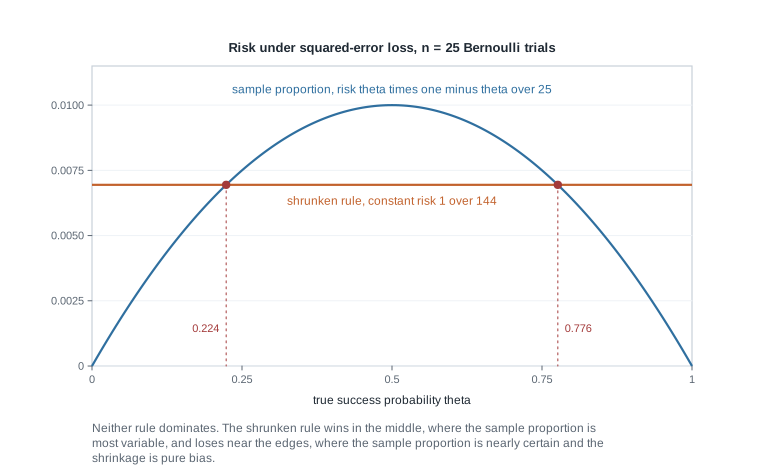
Neither procedure dominates. That is the ordinary situation, not an unlucky one, and Week 1 makes it the organizing fact of the course. The shrunken rule is not an arbitrary invention either: with a Beta\((2.5, 2.5)\) prior the posterior is Beta\((S + 2.5,\, 25 - S + 2.5)\), whose mean is exactly \((S + 2.5)/30\), so this is the Bayes estimator under squared-error loss for that prior. Recall the pattern together with its conditions: under squared-error loss the Bayes rule is the posterior mean whenever the posterior has a finite second moment, under absolute-error loss a posterior median, and under zero-one loss a posterior mode — that last only on a finite parameter space, since for a continuous \(\theta\) every action has expected loss one, and there the mode arrives instead as the limit of a windowed loss, which Week 1 sets out. Averaging the risk function against the prior gives the Bayes risk, a single number, and a rule with constant risk that is Bayes for some prior is minimax, which is the argument Week 14 develops properly.
Projections, quadratic forms, and degrees of freedom
Write the normal linear model as \(Y = X\beta + \varepsilon\) with \(X\) an \(n \times p\) design matrix of full column rank and \(\varepsilon \sim N(0, \sigma^2 I_n)\). The fitted vector is \(\hat{Y} = HY\) with \(H = X(X^{\top}X)^{-1}X^{\top}\). Two properties characterize \(H\) and both are one line of algebra: it is symmetric, and it is idempotent, \(H H = H\). Together these say \(H\) is the orthogonal projection onto the column space of \(X\), and \(I - H\) is the orthogonal projection onto the orthogonal complement. Because \(H(I - H) = 0\), the fitted vector and the residual vector are orthogonal, so squared lengths add.
Two facts follow that Week 8 uses and you should be able to state with conditions. First, if \(Z \sim N(0, I_n)\) and \(A\) is symmetric and idempotent with rank \(r\), then \(Z^{\top} A Z \sim \chi^2_r\); the proof diagonalizes \(A\), whose eigenvalues are all zero or one precisely because it is idempotent, and \(r\) of them are one because rank equals trace for such a matrix. The centering matters as much as the idempotence: this is the central chi-square, and it applies to the residual sum of squares only because \((I - H)X\beta = 0\), so that \((I - H)Y = (I - H)\varepsilon\) has mean zero whatever \(\beta\) is. Second, two such quadratic forms in the same normal vector are independent when the product of their matrices is the zero matrix. Degrees of freedom are ranks of projections, which is why the residual sum of squares in the intercept-only model carries \(n - 1\) of them: with \(J\) the matrix of ones, the residual projection \(I - \frac{1}{n} J\) has rank \(n - 1\).
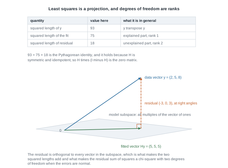
Make it concrete with three numbers. Take \(y = (2, 5, 8)^{\top}\) and the intercept-only model, whose subspace is the span of the vector of ones. Then \(\hat{y} = \bar{y}\mathbf{1} = (5, 5, 5)^{\top}\), the residual is \((-3, 0, 3)^{\top}\), and the squared lengths satisfy \(93 = 75 + 18\). The projection has rank one and the residual projection has rank two, which is the entire content of the phrase “two degrees of freedom” here.
Reproducible simulation as evidence
A calibration claim in this course is checked, not asserted, and the checking instrument is simulation. Three habits make a simulation study evidence rather than anecdote. Set and record a seed, so the run is reproducible. Report the number of replicates, because a Monte Carlo estimate has its own standard error, roughly the replicate standard deviation over the square root of the number of replicates. And keep two uncertainties apart: simulation error shrinks when you add replicates, while the statistical error you are measuring does not, because that one belongs to the sample size \(n\) inside each replicate.
The study below uses the model the first worked example derives in full: independent exponential lifetimes with rate \(\theta\), whose maximum likelihood estimator turns out to be the reciprocal of the sample mean. It draws forty such lifetimes with rate \(0.4\), computes the estimate, repeats twenty thousand times, and compares the simulated bias, standard deviation, and mean squared error against exact formulas.
set.seed(2027)
n     <- 40
theta <- 0.4
reps  <- 20000

one_rep <- function(n, theta) 1 / mean(rexp(n, rate = theta))
hats    <- replicate(reps, one_rep(n, theta))

c(mean = mean(hats),
  bias = mean(hats) - theta,
  sd   = sd(hats),
  mse  = mean((hats - theta)^2))

# exact values for comparison, from the inverse-gamma law of 1 / mean(x)
n * theta / (n - 1)                      # 0.410256, the exact mean
n^2 * theta^2 / ((n - 1)^2 * (n - 2))    # 0.004429, the exact variance
theta^2 / n                              # 0.004000, the asymptotic variance
Because \(\sum_i X_i\) is Gamma with shape \(n\) and rate \(\theta\), the estimator \(\hat\theta = n / \sum_i X_i\) has an inverse-gamma law with exactly computable moments, so this is a rare case where the simulation can be graded against closed form. The exact mean is \(n\theta/(n-1) = 0.410256\), so the bias is \(\theta/(n-1) \approx 0.01026\), upward. The exact standard deviation is \(0.06655\) against the asymptotic \(\theta/\sqrt{n} = 0.06325\), and the exact mean squared error, \(0.004534\), exceeds the asymptotic \(0.004\) by about thirteen percent. A run of twenty thousand replicates gave a mean of \(0.4096\) and a standard deviation of \(0.0660\); the Monte Carlo standard error of that mean is about \(0.0005\), so the agreement is as close as it should be, and a different seed moves the last two digits.
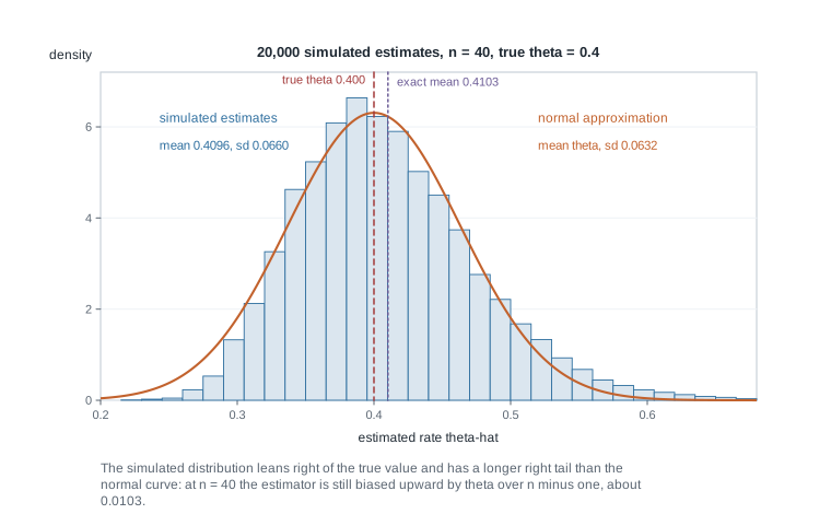
The picture makes the arithmetic visible: the simulated distribution sits a little to the right of the true value and its right tail is heavier than the normal curve allows. Both features shrink as \(n\) grows, and neither is present in the limit statement.
Worked example — the exponential lifetime model end to end
The model and the question. A reliability test runs \(n = 40\) components to failure. Model the lifetimes as independent exponential with rate \(\theta > 0\), density \(f(x; \theta) = \theta e^{-\theta x}\) for \(x > 0\), so the mean lifetime is \(1/\theta\). The observed mean lifetime is \(\bar{x} = 2.5\) hours, so \(\sum_i x_i = 100\). Estimate \(\theta\) and report an interval.
Step 1: the log-likelihood. With independent observations, \(\mathcal{L}(\theta) = \theta^n e^{-\theta \sum_i x_i}\) and
\[ \ell(\theta) \;=\; n \log \theta - \theta \sum_{i=1}^{n} x_i \;=\; 40 \log \theta - 100\,\theta . \]
Step 2: the score and the estimator. Differentiating, \(U(\theta) = n/\theta - \sum_i x_i = 40/\theta - 100\). Setting this to zero gives \(\hat\theta = n / \sum_i x_i = 1/\bar{x} = 0.4\) failures per hour. It is a maximum because \(\ell''(\theta) = -n/\theta^2 < 0\) for every \(\theta > 0\), so \(\ell\) is strictly concave on the whole parameter space and the stationary point is the unique global maximizer.
Step 3: the information. From \(\ell''(\theta) = -n/\theta^2\) we get \(I_n(\theta) = n/\theta^2\) directly, with no expectation needed, since the second derivative is already non-random here. Per observation, \(I_1(\theta) = 1/\theta^2\). At the estimate the observed information is \(40/0.4^2 = 250\), and the estimated standard error is \(1/\sqrt{250} = 0.0632\), the same as \(\hat\theta/\sqrt{n}\).
Step 4: check the regularity before using it. Distinct rates give distinct distributions, so the family is identifiable; the support \((0, \infty)\) does not involve \(\theta\); the parameter space is open, so the true value is interior; \(\theta \mapsto \theta e^{-\theta x}\) is smooth; the family is a one-parameter exponential family with natural parameter \(-\theta\) ranging over an open interval, which licenses differentiation under the integral sign; \(I_1(\theta) = 1/\theta^2\) is finite and positive; and \(\partial^3 \log f(x; \theta) / \partial \theta^3 = 2/\theta^3\) is bounded near \(0.4\) by a constant, so the dominating function the expansion needs may be taken constant and has finite expectation. All seven conditions listed earlier hold, which is why the next step is allowed at all.
Step 5: the approximation and the interval. Therefore \(\sqrt{n}(\hat\theta - \theta) \to_d N(0, \theta^2)\), and the Wald interval at the ninety-five percent level is \(0.4 \pm 1.96 \times 0.0632\), that is \((0.276, 0.524)\).
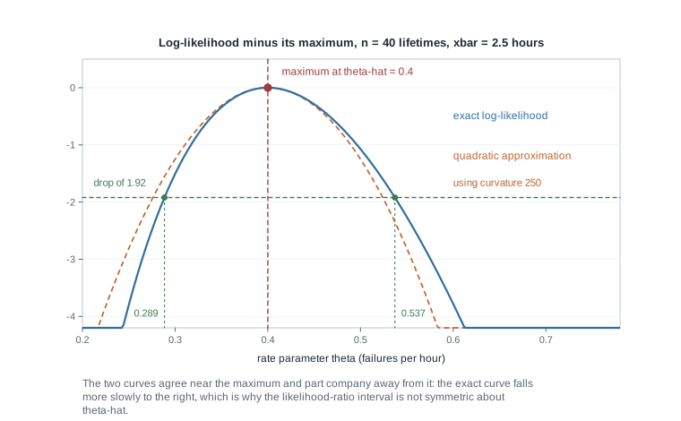
What this licenses and what it does not. The figure shows the quadratic approximation matching the exact log-likelihood near the maximum and falling faster than it on the right; that asymmetry is the same fact the simulation showed. Because this model admits an exact pivot we can measure the damage: \(2\theta \sum_i X_i \sim \chi^2_{2n}\), and inverting it with the chi-square quantiles at eighty degrees of freedom, \(57.15\) and \(106.63\), gives the exact interval \((0.286, 0.533)\).
n <- 40; xbar <- 2.5; hat <- 1 / xbar
hat + c(-1, 1) * qnorm(0.975) * hat / sqrt(n)         # 0.276  0.524
qchisq(c(0.025, 0.975), df = 2 * n) / (2 * n * xbar)  # 0.286  0.533
Both ends of the Wald interval sit low. The interval built from the curve itself, by collecting the \(\theta\) whose log-likelihood is within \(1.92\) of the maximum, runs from \(0.289\) to \(0.537\) and lands much closer to the exact one, which is the first hint of why Week 5 treats the likelihood-ratio and Wald statistics as genuinely different procedures rather than interchangeable ones.
The same reasoning, transferred
Now count colonies on \(n = 60\) culture plates and model the counts as independent Poisson with mean \(\theta\), with observed mean \(\bar{x} = 3.2\). The log-likelihood is \(\ell(\theta) = \bigl(\sum_i x_i\bigr) \log \theta - n\theta\) up to a term free of \(\theta\), the score is \(\sum_i x_i / \theta - n\), and the maximum likelihood estimator is \(\hat\theta = \bar{x} = 3.2\). Here \(\ell''(\theta) = -\sum_i x_i/\theta^2\) is random rather than constant, so the information comes from an expectation this time: \(I_1(\theta) = E_\theta(X)/\theta^2 = 1/\theta\). The estimated standard error is \(\sqrt{\hat\theta/n} = \sqrt{3.2/60} = 0.231\), giving the Wald interval \((2.747, 3.653)\).
What stayed the same: a one-parameter exponential family, a score linear in the sufficient statistic \(\sum_i X_i\), a strictly concave log-likelihood with a unique interior maximizer, and the same seven regularity conditions verified the same way, the third derivative \(2\sum_i x_i / \theta^3\) being bounded near \(3.2\) by a multiple of \(\sum_i x_i\), whose expectation is finite. What changed: the data are discrete, the information is \(1/\theta\) rather than \(1/\theta^2\), and the estimator is the sample mean itself rather than a nonlinear function of it. Discreteness has a further consequence Week 4 takes up in earnest: exact intervals in discrete models are conservative, because no cutoff achieves the nominal level precisely.
Second worked example — a smooth function of the estimator
Return to the reliability test with \(n = 40\), \(\bar{x} = 2.5\), \(\hat\theta = 0.4\). Engineers rarely want a rate; they want a mean lifetime, or the probability that a component survives a stated warranty period. Both are smooth functions of \(\theta\), so both are delta-method problems, and they behave differently.
Facet one: the mean lifetime. Let \(g(\theta) = 1/\theta\), so \(g'(\theta) = -1/\theta^2\). The asymptotic variance of \(\sqrt{n}(\hat\mu - \mu)\) is \(g'(\theta)^2 \theta^2 = 1/\theta^2\), hence \(\operatorname{Var}(\hat\mu) \approx 1/(n\theta^2) = \mu^2/n\). With \(\hat\mu = 1/\hat\theta = \bar{x} = 2.5\) this gives \(6.25/40 = 0.15625\) and a standard error of \(0.395\), so the interval is \(2.5 \pm 1.96 \times 0.395 = (1.725, 3.275)\). Here is a useful check: \(\hat\mu\) is just \(\bar{X}\), whose exact variance is \(\operatorname{Var}(X)/n = \mu^2/n\), so the delta method reproduced the exact variance rather than approximating it.
Facet two: a survival probability. Let \(\psi = P_\theta(X > 3) = e^{-3\theta}\), the chance a component lasts past three hours, so \(g(\theta) = e^{-3\theta}\) and \(g'(\theta) = -3e^{-3\theta}\). The estimate is \(\hat\psi = e^{-1.2} = 0.301\). The approximate variance of \(\hat\psi\) is \(g'(\theta)^2 \theta^2 / n = 9 e^{-2.4} \times 0.16/40 = 0.003266\), evaluated at \(\hat\theta\), so the standard error is \(0.0571\) and the interval is \(0.301 \pm 1.96 \times 0.0571 = (0.189, 0.413)\).
Facet three: the same quantity on another scale. Work instead with \(\log \psi = -3\theta\), whose approximate variance is \(9\theta^2/n = 0.036\) and standard deviation \(0.190\). The interval for \(\log\psi\) is \(-1.2 \pm 1.96 \times 0.190 = (-1.572, -0.828)\), and exponentiating gives \((0.208, 0.437)\) for \(\psi\). Two applications of the same theorem to the same data have produced two different intervals, and neither is a computational mistake.
What this licenses and what it does not. The delta method is a statement about a limit, and different smooth reparameterizations reach that limit at different speeds. The log-scale interval is preferable here because back-transforming keeps both endpoints positive whatever the data do: the log removes the boundary at zero, and a symmetric interval built directly on \(\psi\) has no such protection, its lower end at \(n = 5\), where the standard error rises to \(0.162\), falling below zero, which is not a probability. Be exact about how far that argument reaches. The log does not remove the other boundary: \(\log\psi\) is still capped above by zero, and the scale genuinely unconstrained for a probability is the logit \(\log\{\psi/(1 - \psi)\}\), which is what you would want if \(\hat\psi\) sat near one. The approximation is also poor whenever \(g'(\theta)\) is near zero, where the expansion changes character, as shown earlier. Week 5 returns to this sensitivity under the name of the Wald statistic’s dependence on parameterization, and shows that the likelihood-ratio statistic does not share it.
The misreading to avoid
The misreading sounds like this: “The maximum likelihood estimator is unbiased and normally distributed with variance the inverse of the Fisher information, so with \(n = 40\) I can write down a symmetric interval and be done.” Every clause is a limit statement read as a finite-sample promise, and this page has already priced the error: at \(n = 40\) the exponential rate estimator is biased upward by about two and a half percent, its exact standard deviation and mean squared error exceed the asymptotic values by about five and thirteen percent, and its distribution is right-skewed, which is why the exact interval \((0.286, 0.533)\) sits to the right of the Wald interval \((0.276, 0.524)\) rather than merely being wider. The theorem was never wrong. It described a sequence, and forty is not infinity.
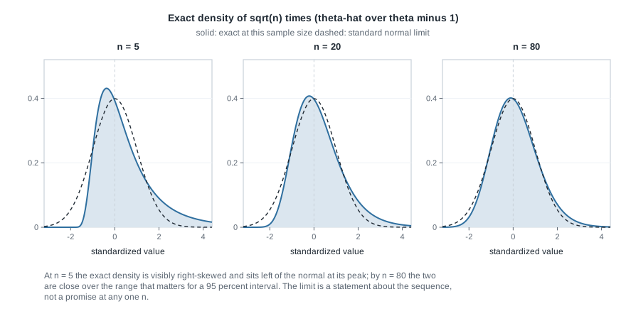
The figure is the honest version of the claim. At \(n = 5\) the exact density of the standardized estimator is strongly right-skewed and its peak sits left of the normal’s; by \(n = 80\) the two nearly coincide over the range a ninety-five percent interval uses. The only way to learn what the limit delivers at your \(n\) is to compare it against something exact or simulated, as above.
Two smaller misreadings travel with the large one. The first treats the likelihood as a distribution over \(\theta\), reading “the likelihood at \(\theta_1\) is twice the likelihood at \(\theta_2\)” as “\(\theta_1\) is twice as probable”. A probability statement about \(\theta\) requires a prior; without one the likelihood ratio is evidence, not probability. The second reads a large Fisher information as a promise about the realized data set. Information is an expectation over repeated samples at a fixed \(\theta\), and a particular sample can be uninformative even when \(I_n(\theta)\) is large, which is why the observed information, the curvature at the realized maximum, is often the better standard-error ingredient.
Practice on your own
These are for self-checking as you read, not for submission. Work them with a pencil first and only then with R.
- The Bernoulli pipeline. For \(X_1, \dots, X_n\) independent Bernoulli with success probability \(\theta\), write the log-likelihood, derive the score, solve for \(\hat\theta\), and obtain \(I_1(\theta) = 1 / \bigl(\theta(1-\theta)\bigr)\) from both information identities. Confirm they agree, then say which of the seven regularity conditions you would have to check again if \(\theta\) were allowed to equal zero.
- A condition that fails. For \(X_1, \dots, X_n\) uniform on \((0, \theta)\), show by direct calculation that \(E_\theta[\partial \log f(X;\theta) / \partial \theta] \neq 0\), identify which interchange is invalid, derive the exact distribution of \(X_{(n)}\), and confirm the exponential limit law stated earlier by letting \(n\) grow in the exact survival probability.
- A variance-stabilizing transformation. Apply the delta method to \(\log \hat\theta\) in the exponential model and show that its asymptotic variance is \(1/n\), free of \(\theta\). Build the interval for \(\theta\) by back-transforming, compare it with the Wald and exact intervals above, and explain in one sentence why it is not symmetric about \(0.4\).
- A simulation you can grade. Rerun the estimator study at \(n = 10\) and at \(n = 160\), and check whether the simulated bias and mean squared error track the exact \(\theta/(n-1)\) and \(n^2\theta^2 / \bigl((n-1)^2(n-2)\bigr) + \theta^2/(n-1)^2\). Report the Monte Carlo standard error beside each estimate, and state the sample size at which you would use the normal approximation.
- Geometry. For a one-way layout with two groups of sizes three and four, write the design matrix, verify that \(H\) is symmetric and idempotent, compute its rank from its trace, and state the degrees of freedom of the residual projection without counting parameters.
Where to read more
- MIT OpenCourseWare 18.655 Mathematical Statistics is the closest open graduate treatment, and its opening lectures on models, likelihood, and decision theory are worth skimming now.
- Penn State STAT 415 Introduction to Mathematical Statistics is the gentler open reference and the better first stop if a strand above felt unfamiliar rather than rusty.
- The optional Hogg, McKean, and Craig alignment for this week is Chapters 4 through 7, together with Chapter 11, all as review. The text is optional throughout this course and is never required to be purchased; availability and licence terms for every source listed here are still being confirmed.
- Computing runs on The R Project for Statistical Computing and Quarto, and nothing beyond those two is needed all semester.
- The course pages: the syllabus, the schedule, the resources overview, and the notes index.
Where this goes next
Week 1 takes the loss and risk material from this page and makes it the frame for everything else. Instead of treating risk as one property of an estimator among many, it treats a statistical procedure as a decision rule and asks how two procedures are compared when their risk functions cross, as the two curves above did. The partial ordering that comparison induces, and the two standard ways of collapsing a risk function into a single number, are what the rest of the course argues with.
Read Week 1 — Statistical decisions, actions, loss, and risk next, and return to the notes index for the full sequence. If any strand here felt unfamiliar rather than rusty, do the corresponding bridge reading during these first two weeks: the likelihood machinery reappears in Week 5, the projection geometry in Week 8, and loss and risk in Weeks 1 and 14, and each of those units assumes what this page reviewed.