Week 15 — Jordan canonical form and the classification of operators
Where this week starts
Week 4 asked a question that this page settles. Once you fix an ordered basis, an operator becomes a matrix; change the basis and the matrix changes by \(A \mapsto P^{-1}AP\). Which features of the array survive that change? For matrix equivalence, where both bases are free to move, Week 4 gave a complete invariant in one number: rank, and the rank normal form as a representative for each class. For similarity, where only one basis moves, the same page could list invariants — rank, trace, determinant, and from Week 10 the characteristic polynomial — without ever showing the list was complete. It was not complete, and Week 13 exhibited the failure: \(\operatorname{diag}(2,2)\) and the two-by-two block with a \(1\) above the diagonal share every one of those invariants and are not similar.
Weeks 13 and 14 then built what the missing invariant needs. The minimal polynomial \(m_T\) separated that particular pair but not all pairs, since two four-by-four matrices can agree on both \(p_T\) and \(m_T\) and still be different operators. Week 14 supplied the finer data: for each eigenvalue \(\lambda\), the sequence of ranks of the powers of \(T - \lambda I\), from which the lengths of the cyclic chains fall out by subtraction. This week assembles those chains into a single matrix, proves it is essentially the only one of its shape, and proves the list of block sizes is a complete invariant for similarity whenever \(p_T\) splits over the field.
The object is the Jordan canonical form: a block diagonal matrix whose diagonal blocks are \(J_k(\lambda)\), each carrying one eigenvalue down its diagonal and ones directly above. The theorem has two halves. Existence says every operator on a finite-dimensional space whose characteristic polynomial splits is similar to such a matrix — that half is Week 14’s primary decomposition and cyclic decomposition, put end to end. Uniqueness says the multiset of blocks is determined by the operator, and it follows from a single computation: the ranks of the powers of \(J - \lambda I\) can be read straight off the block sizes, and rank is a similarity invariant.
By the end of the page three things should feel different. A defective operator should stop looking like an anomaly and start looking like a point in a finite list you can enumerate. The question are these two matrices similar should become a computation rather than a search for a conjugating matrix. And the hypothesis that \(p_T\) splits should feel like the load-bearing wall it is: the moment it is removed — over \(\mathbb{R}\), over \(\mathbb{Q}\), over \(\mathbb{F}_2\) — the classification stops.
Why this matters beyond the definition
Here is a claim people make and then act on: two matrices with the same characteristic polynomial and the same minimal polynomial are the same operator up to a change of basis. It is the natural thing to believe after Week 13, because \(m_T\) repaired the first counterexample. The second worked example below breaks it in dimension four. Two operators on \(\mathbb{C}^4\) both have \(p_T(t) = (t-3)^4\) and both have \(m_T(t) = (t-3)^2\), yet one has a two-dimensional eigenspace and the other a three-dimensional one, so they cannot be similar. Anyone who concluded similarity from the two polynomials has silently identified two different operators, and every quantity computed downstream — the dimension of a fixed subspace, the number of independent equilibrium directions in a linear system — comes out wrong.
The second stake is that the classification is finite and enumerable. Over \(\mathbb{C}\) the similarity classes of \(n \times n\) matrices with a single eigenvalue \(\lambda\) correspond exactly to the partitions of \(n\): five of them when \(n = 4\), and no more. That is why a question like “how many essentially different four-by-four nilpotent matrices are there” has an exact numerical response rather than an evasion.
What you will be able to do
- Define \(J_k(\lambda)\) and a Jordan matrix, and compute \(p\), \(m\), the eigenspace dimension, and every \(\operatorname{rank}(J - \lambda I)^{k}\) directly from a list of block sizes.
- State the Jordan canonical form theorem with the hypothesis that \(V\) is finite-dimensional and \(p_T\) splits over \(F\), and assemble the existence half from Week 14’s primary and cyclic decompositions.
- Prove that the multiset of blocks is unique, by showing the rank differences \(\operatorname{rank}(T-\lambda I)^{k-1} - \operatorname{rank}(T-\lambda I)^{k}\) count the blocks of size at least \(k\).
- Decide whether two explicit complex matrices are similar by computing rank sequences, without ever searching for a conjugating matrix.
- Enumerate every Jordan form with a prescribed characteristic polynomial, and identify which pairs the polynomials alone fail to separate.
- Exhibit an operator over \(\mathbb{R}\) with no Jordan form at all, and say precisely which hypothesis it violates.
Terms and notation worth fixing
| Symbol or term | What it means on this page |
|---|---|
| \(J_k(\lambda)\) | the \(k \times k\) Jordan block: \(\lambda\) down the diagonal, \(1\) on the superdiagonal, \(0\) elsewhere |
| Jordan matrix | a block diagonal matrix every one of whose diagonal blocks is some \(J_k(\lambda)\) |
| a Jordan form of \(T\) | a Jordan matrix similar to \(T\); the theorem makes it unique up to the order of its blocks |
| block data at \(\lambda\) | the multiset of sizes of the blocks carrying the eigenvalue \(\lambda\), written as a partition |
| \(d_k(\lambda)\) | \(\operatorname{rank}(T - \lambda I)^{k-1} - \operatorname{rank}(T - \lambda I)^{k}\), with \((T - \lambda I)^0 = I\) |
| \(p_T\) splits over \(F\) | \(p_T(t) = (t - \lambda_1)^{m_1}\cdots(t-\lambda_r)^{m_r}\) with every \(\lambda_i\) in \(F\) |
| \(\operatorname{alg}(\lambda)\), \(\operatorname{geo}(\lambda)\) | the multiplicity of \(\lambda\) as a root of \(p_T\), and \(\dim E_{\lambda}\), as in Week 11 |
| \(A \sim B\) | \(B = P^{-1}AP\) for some invertible \(P\): the similarity relation of Week 4 |
Assembling the Jordan canonical form
Two theorems from Week 14 do all the work. The primary decomposition splits \(V\) into invariant pieces on which \(T\) is a scalar plus a nilpotent operator; the cyclic decomposition splits each nilpotent operator into chains. What remains is to order the bases and name the matrix that results.
Jordan blocks and Jordan matrices
Definition. For \(k \ge 1\) and \(\lambda \in F\), the Jordan block \(J_k(\lambda)\) is the \(k \times k\) matrix over \(F\) with \(\lambda\) in every diagonal position, \(1\) in every position directly above the diagonal, and \(0\) everywhere else. So \(J_1(\lambda) = (\lambda)\), and \(J_3(\lambda)\) is the array with rows \((\lambda, 1, 0)\), \((0, \lambda, 1)\), \((0, 0, \lambda)\). A Jordan matrix is a block diagonal matrix whose diagonal blocks are Jordan blocks; different blocks may carry the same eigenvalue or different ones.
Everything about a single block is immediate, and the uniqueness proof consumes all of it. Put \(N = J_k(\lambda) - \lambda I = J_k(0)\), the block with zeros on the diagonal. Then \(N\) moves each standard basis vector one place down the list, \(e_j \mapsto e_{j-1}\), and kills \(e_1\); so \(N^{j}\) moves each vector \(j\) places, \(N^{k} = 0\), \(N^{k-1} \ne 0\), and
\[\operatorname{rank} N^{j} = \max(k - j, \, 0) \quad \text{for every } j \ge 0 .\]
Consequently \(\dim \ker (J_k(\lambda) - \lambda I) = 1\): a Jordan block contributes exactly one independent eigenvector, no matter how large it is. Since \(J_k(\lambda)\) is upper triangular with \(\lambda\) repeated on the diagonal, its characteristic polynomial is \((t - \lambda)^{k}\), and its minimal polynomial is \((t-\lambda)^{k}\) as well, because \(N^{k} = 0\) and no smaller power vanishes. Finally, if \(\mu \ne \lambda\) then \(J_k(\lambda) - \mu I\) is upper triangular with the nonzero scalar \(\lambda - \mu\) repeated down its diagonal, hence invertible, and so is each of its powers; that block contributes its full \(k\) to \(\operatorname{rank}(J - \mu I)^{j}\) for every \(j\).
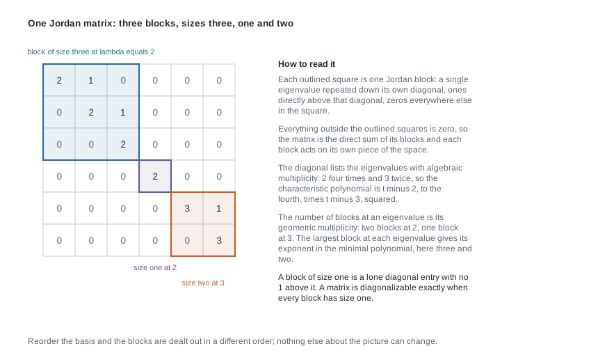
The figure is the Jordan matrix the worked example below produces. Read the diagonal and you have \(p(t) = (t-2)^4(t-3)^2\), since the matrix is upper triangular. Count the outlined squares carrying \(2\) and you have \(\operatorname{geo}(2) = 2\); count the squares carrying \(3\) and you have \(\operatorname{geo}(3) = 1\). Take the largest square at each eigenvalue and you have the exponents in \(m(t) = (t-2)^3(t-3)^2\). The only choice made in drawing it was the order in which the three squares were dealt along the diagonal.
Existence: putting Week 14 together
Theorem (Jordan canonical form, existence). Let \(V\) be a finite-dimensional vector space over a field \(F\) with \(\dim V = n \ge 1\), let \(T \in \mathcal{L}(V)\), and suppose the characteristic polynomial \(p_T(t) = \det(tI - T)\) splits over \(F\). Then \(V\) has an ordered basis \(\mathcal{B}\) in which \([T]_{\mathcal{B} \leftarrow \mathcal{B}}\) is a Jordan matrix. Equivalently, every \(A \in M_n(F)\) whose characteristic polynomial splits over \(F\) is similar to a Jordan matrix.
Argument. Write \(p_T(t) = (t - \lambda_1)^{m_1}\cdots(t-\lambda_r)^{m_r}\) with the \(\lambda_i\) distinct and \(m_1 + \cdots + m_r = n\). Week 14’s primary decomposition theorem, which needs exactly the two hypotheses just stated, gives
\[V = G_{\lambda_1} \oplus \cdots \oplus G_{\lambda_r}, \qquad \dim G_{\lambda_i} = m_i ,\]
with each \(G_{\lambda_i}\) invariant under \(T\) and with \(N_i = (T - \lambda_i I)|_{G_{\lambda_i}}\) nilpotent.
Fix one \(i\) and work inside \(G_{\lambda_i}\), a finite-dimensional space on which \(N_i\) is a nilpotent operator. Week 14’s cyclic decomposition theorem writes \(G_{\lambda_i} = Z(v_{i1}) \oplus \cdots \oplus Z(v_{is_i})\), where each \(Z(v)\) is the span of a chain \(v, N_i v, \dots, N_i^{p-1}v\) with \(N_i^{p} v = 0\). Order each chain from the bottom up, as \(\big(N_i^{p-1}v, \dots, N_i v, v\big)\). Week 14’s chain lemma says the matrix of \(N_i\) on \(Z(v)\) in that order is \(J_p(0)\). Now \(T\) restricted to \(Z(v)\) equals \(\lambda_i I + N_i\) there, and the identity has matrix \(I_p\) in any basis, so
\[[T|_{Z(v)}] = \lambda_i I_p + J_p(0) = J_p(\lambda_i) .\]
Concatenate: take the chain bases of \(G_{\lambda_1}\) in order, then those of \(G_{\lambda_2}\), and so on. A list formed by concatenating bases of the summands of a direct sum is a basis of the whole, by Week 1’s uniqueness of decomposition together with Week 2’s dimension count. Each \(Z(v_{ij})\) is invariant under \(T\), since it is invariant under \(N_i\) and under \(\lambda_i I\), so no basis vector is sent outside its own chain and the matrix of \(T\) in \(\mathcal{B}\) is block diagonal with the blocks \(J_{p_{ij}}(\lambda_i)\) down the diagonal. That is a Jordan matrix.
Nothing here is new mathematics; what is new is the packaging. Name the two places a hypothesis is spent. Finite-dimensionality is used twice over — the primary decomposition needs \(\dim V\) finite to make \(G_{\lambda} = \ker (T-\lambda I)^{\dim V}\) meaningful and to run rank-nullity, and the cyclic decomposition inducts on the dimension. Splitting is used once, decisively: without it the generalized eigenspaces need not fill \(V\), and the direct sum in the first display is simply false.
Reading the block sizes off the ranks
Existence produces a Jordan matrix. To know it is the Jordan matrix we compute what an operator can see; that computation also gives the recipe for finding the blocks without constructing a basis.
Lemma (ranks of a Jordan matrix). Let \(J\) be a Jordan matrix over \(F\) with blocks \(J_{p_1}(\mu_1), \dots, J_{p_q}(\mu_q)\), and fix \(\lambda \in F\). Then for every integer \(k \ge 0\),
\[\operatorname{rank}(J - \lambda I)^{k} \;=\; \sum_{j \,:\, \mu_j \ne \lambda} p_j \;+\; \sum_{j \,:\, \mu_j = \lambda} \max(p_j - k, \, 0) .\]
Argument. Subtracting \(\lambda I\) and raising to the \(k\)-th power are both performed blockwise, because \(J\) is block diagonal, and the rank of a block diagonal matrix is the sum of the ranks of its blocks — the columns coming from different blocks have disjoint supports, so no combination across blocks can be nontrivial. On a block with \(\mu_j \ne \lambda\) the matrix \((J_{p_j}(\mu_j) - \lambda I)^{k}\) is invertible, as noted above, contributing \(p_j\). On a block with \(\mu_j = \lambda\) we get \(J_{p_j}(0)^{k}\), of rank \(\max(p_j - k, 0)\).
Theorem (the counting rule). Let \(V\) be finite-dimensional over \(F\), let \(T \in \mathcal{L}(V)\) have a Jordan matrix \(J\), and let \(\lambda \in F\). For \(k \ge 1\) put
\[d_k(\lambda) = \operatorname{rank}(T - \lambda I)^{k-1} - \operatorname{rank}(T - \lambda I)^{k} .\]
Then \(d_k(\lambda)\) is the number of blocks of \(J\) carrying \(\lambda\) of size at least \(k\), and \(d_k(\lambda) - d_{k+1}(\lambda)\) is the number of size exactly \(k\).
Argument. Similar matrices have equal rank at every power, since \((P^{-1}AP)^{k} = P^{-1}A^{k}P\) and multiplying by invertible matrices changes no rank — that is Week 4. So the ranks of the powers of \(T - \lambda I\) agree with those of \(J - \lambda I\), and the lemma applies. In the difference \(d_k(\lambda)\), the first sum in the lemma is a constant independent of \(k\) and cancels. What survives is
\[d_k(\lambda) = \sum_{j \,:\, \mu_j = \lambda} \big[\max(p_j - k + 1, 0) - \max(p_j - k, 0)\big] ,\]
and each bracket equals \(1\) when \(p_j \ge k\) and \(0\) otherwise. Subtracting the same identity at \(k+1\) leaves the blocks of size exactly \(k\).
This is Week 14’s counting rule for chains restated in the language of blocks; a chain of length \(p\) produces a block of size \(p\). Three corollaries are the ones you use. Taking \(k = 1\), the number of blocks at \(\lambda\) is \(n - \operatorname{rank}(T - \lambda I) = \dim E_{\lambda} = \operatorname{geo}(\lambda)\). Summing all block sizes at \(\lambda\) gives \(\dim G_{\lambda} = \operatorname{alg}(\lambda)\). And the largest block size at \(\lambda\) is the exponent of \((t - \lambda)\) in \(m_T\), because \((J - \lambda I)^{k}\) kills the \(\lambda\)-blocks exactly when \(k\) reaches the largest of them.
Similarity is decided by Jordan type
The rule just proved computes the blocks from the operator. Since it uses only ranks, and ranks cannot tell two similar operators apart, the blocks are an invariant. This section shows they are a complete invariant: the list of blocks is not merely something similar matrices share but everything they share.
Uniqueness of the block multiset
Theorem (uniqueness). Let \(V\) be finite-dimensional over \(F\) and \(T \in \mathcal{L}(V)\), and suppose \(J\) and \(J'\) are Jordan matrices both similar to \(T\). Then \(J\) and \(J'\) have the same blocks, with the same multiplicities; they differ at most in the order in which those blocks are listed.
Argument. A scalar \(\lambda\) occurs on the diagonal of a Jordan matrix similar to \(T\) exactly when \(\lambda\) is a root of \(p_T\), since the Jordan matrix is triangular and similar matrices have the same characteristic polynomial. So \(J\) and \(J'\) use the same set of eigenvalues. Fix one, \(\lambda\). Both \(J\) and \(J'\) are similar to \(T\), so for every \(k\) we have \(\operatorname{rank}(J - \lambda I)^{k} = \operatorname{rank}(T - \lambda I)^{k} = \operatorname{rank}(J' - \lambda I)^{k}\). By the counting rule the number of blocks at \(\lambda\) of size exactly \(k\) equals \(d_k(\lambda) - d_{k+1}(\lambda)\) in both matrices, and that quantity was computed from \(T\) alone. So the two matrices carry the same number of blocks of each size at each eigenvalue, which is what the multiset claim says.
Conversely, reordering the blocks of a Jordan matrix does produce a similar matrix: permuting the basis vectors so that the chains appear in a different order changes the matrix by conjugation with the corresponding permutation matrix, which is invertible. So “unique up to the order of the blocks” is exactly right.
Theorem (similarity is decided by Jordan type). Let \(A, B \in M_n(\mathbb{C})\). Then \(A\) and \(B\) are similar if and only if they have the same Jordan form up to the order of blocks.
Argument. Both directions are now short. Over \(\mathbb{C}\) every polynomial splits, so existence supplies Jordan matrices \(J_A \sim A\) and \(J_B \sim B\). If \(A \sim B\) then \(J_A \sim J_B\), and both are Jordan matrices similar to the same operator, so uniqueness makes their block multisets equal. If instead the block multisets are equal, then \(J_A\) and \(J_B\) differ by a permutation of blocks, hence \(J_A \sim J_B\); since similarity is transitive and symmetric — it is conjugation by a group of invertible matrices — \(A \sim J_A \sim J_B \sim B\).
That closes the question Week 4 opened. Two matrices are the same operator in different bases precisely when their block data agree, and that data comes from finitely many rank calculations. Deciding similarity never requires finding \(P\): compute \(\operatorname{rank}(A - \lambda I)^{k}\) and \(\operatorname{rank}(B - \lambda I)^{k}\) for the eigenvalues and for \(k\) up to \(n\), and compare integers.
What the classification does not settle
The theorem is sharp, and it has edges. The first is the field. Over \(\mathbb{R}\) the quarter-turn rotation of the plane, \(R = \begin{pmatrix} 0 & -1 \\ 1 & 0 \end{pmatrix}\), has \(p_R(t) = t^2 + 1\), which has no real root, so \(R\) has no real eigenvalue, no real eigenvector, and no real Jordan form — a Jordan matrix over \(\mathbb{R}\) would be triangular with real eigenvalues on the diagonal, and \(R\) has none. There is a substitute, the real canonical form, in which the blocks for a conjugate pair \(a \pm bi\) are built from two-by-two real blocks \(\begin{pmatrix} a & -b \\ b & a \end{pmatrix}\); this course states its existence and does not develop it. Over \(\mathbb{Q}\) and over \(\mathbb{F}_2\) the same obstruction appears with different polynomials, as Week 14 showed, and the general repair is the rational canonical form, which needs no splitting at all. Passing to \(\mathbb{C}\) is the repair this course uses: \(R\) over \(\mathbb{C}\) has eigenvalues \(i\) and \(-i\), each simple, so its Jordan form is \(\operatorname{diag}(i, -i)\).
The second edge is that similar is not equal. The Jordan form of \(A\) tells you what the operator does; it does not tell you what \(A\) looks like, and recovering \(A\) from \(J\) needs the conjugating matrix \(P\), whose columns are the chain basis. Two matrices with the same Jordan form can have no entry in common.
The third edge surprises people. The Jordan form is not a continuous function of the entries. Compare \(\begin{pmatrix} 2 & 1 \\ 0 & 2 \end{pmatrix}\), whose form is the single block \(J_2(2)\), with \(\begin{pmatrix} 2 & 1 \\ 0 & 2 + \varepsilon \end{pmatrix}\) for any \(\varepsilon \ne 0\): the latter has two distinct eigenvalues, hence two independent eigenvectors by Week 11, hence Jordan form \(\operatorname{diag}(2, 2+\varepsilon)\) with two blocks of size one. Arbitrarily small changes in the entries change the block structure completely. The classification is a theorem about exact arithmetic over a field, and treating it as a numerical algorithm on measured data is a category error.
Worked example — a six by six matrix put into Jordan form
Work over \(\mathbb{C}\) with \(V = \mathbb{C}^6\) and
\[A = \begin{pmatrix} 2 & 1 & 1 & 1 & 0 & 0 \\ 0 & 2 & 1 & 1 & 0 & 0 \\ 0 & 0 & 2 & 0 & 0 & 1 \\ 0 & 0 & 0 & 2 & 1 & 0 \\ 0 & 0 & 0 & 0 & 3 & 1 \\ 0 & 0 & 0 & 0 & 0 & 3 \end{pmatrix} .\]
The task: find the Jordan form of \(A\) and a basis realising it, using nothing but ranks.
Step 1. The characteristic polynomial. \(A\) is upper triangular, so \(tI - A\) is upper triangular with diagonal entries \(t-2, t-2, t-2, t-2, t-3, t-3\), and the determinant of a triangular matrix is the product of its diagonal. Hence \(p_A(t) = (t-2)^4(t-3)^2\), which splits over \(\mathbb{Q}\) already, so the existence theorem applies without enlarging the field. Then \(\operatorname{alg}(2) = 4\) and \(\operatorname{alg}(3) = 2\). As a check, the trace is \(2+2+2+2+3+3 = 14\), and the sum of the roots with multiplicity is \(8 + 6 = 14\).
Step 2. The rank sequence at \(\lambda = 2\). Put \(N = A - 2I\). Naming its columns \(c_1, \dots, c_6\) is the efficient way to raise it to powers, since \(Nx = \sum_j x_j c_j\). Reading them off,
\[c_1 = 0, \quad c_2 = e_1, \quad c_3 = c_4 = e_1 + e_2, \quad c_5 = e_4 + e_5, \quad c_6 = e_3 + e_5 + e_6 .\]
The nonzero distinct ones are \(e_1\), \(e_1 + e_2\), \(e_4 + e_5\), \(e_3 + e_5 + e_6\); the first two are independent and supported in coordinates one and two, the last two are independent of them and of each other, so \(\operatorname{rank} N = 4\). For \(N^2\), apply \(N\) to each column: \(Nc_2 = Ne_1 = c_1 = 0\), \(Nc_3 = Nc_4 = c_1 + c_2 = e_1\), \(Nc_5 = c_4 + c_5 = (1,1,0,1,1,0)^{\mathsf{T}}\), and \(Nc_6 = c_3 + c_5 + c_6 = (1,1,1,1,2,1)^{\mathsf{T}}\). Those last three vectors are independent — look at coordinate six, then coordinate four, then coordinate one — so \(\operatorname{rank} N^2 = 3\). One more step: \(Ne_1 = 0\), while
\[N(1,1,0,1,1,0)^{\mathsf{T}} = c_2 + c_4 + c_5 = (2,1,0,1,1,0)^{\mathsf{T}}, \qquad N(1,1,1,1,2,1)^{\mathsf{T}} = c_2 + c_3 + c_4 + 2c_5 + c_6 = (3,2,1,2,3,1)^{\mathsf{T}} ,\]
two independent vectors, so \(\operatorname{rank} N^3 = 2\). Since \(\dim \ker N^3 = 6 - 2 = 4 = \operatorname{alg}(2) = \dim G_2\) and \(\ker N^3 \subseteq G_2\), the kernel chain has already reached \(G_2\), so by Week 14’s stabilisation lemma \(\operatorname{rank} N^4 = 2\) as well.
Step 3. Blocks at \(\lambda = 2\). The rank sequence is \(6, 4, 3, 2, 2\). The counting rule gives \(d_1 = 6-4 = 2\) blocks of size at least one, \(d_2 = 4-3 = 1\) of size at least two, \(d_3 = 3-2 = 1\) of size at least three, and \(d_4 = 2-2 = 0\) of size at least four. Differencing once more: one block of size exactly one, none of size two, one of size three. So the blocks at \(2\) are \(J_3(2)\) and \(J_1(2)\), and \(3 + 1 = 4 = \operatorname{alg}(2)\), as it must.
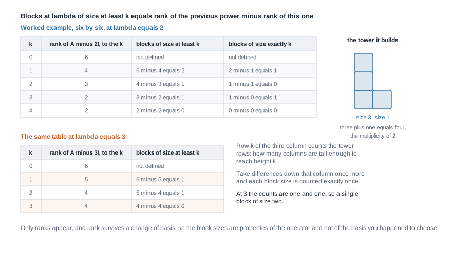
The figure carries both rank sequences and the tower they build. Read the third column downward and you count how many columns reach height \(k\); read the fourth and each block is counted once, at its own height. The tower has total area four, matching \(\operatorname{alg}(2)\), and two columns, matching \(\operatorname{geo}(2) = 6 - \operatorname{rank} N = 2\). Every entry is a rank, so the shape beside the tables belongs to the operator rather than the matrix.
Step 4. Blocks at \(\lambda = 3\). Put \(S = A - 3I\). The top-left four-by-four corner of \(S\) is upper triangular with \(-1\) down its diagonal, hence invertible, and the bottom-left two-by-four corner is zero. Write \(r_1, \dots, r_6\) for the rows of \(S\) and suppose \(a_1 r_1 + \cdots + a_5 r_5 = 0\). Row five is \((0,0,0,0,0,1)\), so it contributes nothing in the first four coordinates; reading the relation there leaves \((a_1, a_2, a_3, a_4)\) multiplied on the right by the invertible top-left four-by-four corner and equal to zero, which forces \(a_1 = a_2 = a_3 = a_4 = 0\). What is left of the relation is \(a_5(0,0,0,0,0,1) = 0\), so \(a_5 = 0\) as well. The first five rows are therefore independent, and row six is zero, so \(\operatorname{rank} S = 5\). For higher powers write \(A\) in block form with corners \(M\) (four-by-four, upper left) and \(C = \begin{pmatrix} 3 & 1 \\ 0 & 3 \end{pmatrix}\) (two-by-two, lower right), the lower left corner being zero. Then \(S^{k}\) is block upper triangular with corners \((M - 3I)^{k}\) and \((C - 3I)^{k}\). Now \((C-3I)^2 = 0\) and \(M - 3I\) is invertible, so for \(k \ge 2\) the last two rows of \(S^{k}\) vanish while the first four columns hold the invertible \((M-3I)^{k}\): \(\operatorname{rank} S^{k} = 4\) for every \(k \ge 2\). The sequence is \(6, 5, 4, 4\), giving \(d_1 = 1\), \(d_2 = 1\), \(d_3 = 0\): a single block \(J_2(3)\).
Step 5. The form, and a basis for it. Collecting Steps 3 and 4,
\[J = J_3(2) \oplus J_1(2) \oplus J_2(3), \qquad m_A(t) = (t-2)^3(t-3)^2 ,\]
the minimal polynomial coming from the largest block at each eigenvalue. For a basis, first note \(G_2 = \ker N^3\): from Step 2, \(N^3x = x_5(2,1,0,1,1,0)^{\mathsf{T}} + x_6(3,2,1,2,3,1)^{\mathsf{T}}\), and those two vectors are independent, so \(N^3x = 0\) exactly when \(x_5 = x_6 = 0\). Inside that span, \(N^2x = (x_3 + x_4)e_1\), so \(v = e_3\) generates a chain of length three:
\[v = e_3, \qquad Nv = c_3 = (1,1,0,0,0,0)^{\mathsf{T}}, \qquad N^2v = e_1, \qquad N^3 v = 0 .\]
Solving \(Nx = 0\) coordinate by coordinate gives \(x_6 = 0\), then \(x_5 = 0\), then \(x_3 + x_4 = 0\), then \(x_2 = 0\), so \(\ker N = \operatorname{span}(e_1, \, e_3 - e_4)\), of dimension two as the rank predicted. Take \(u = e_3 - e_4\) for the short chain; it is independent of \(N^2 v = e_1\). For \(\lambda = 3\), note that \(N\) is invertible on \(G_3\) and zero on \(G_2\) after three steps, so \(G_3 = \operatorname{im} N^3\), spanned by the two vectors displayed above. Take \(w = (3,2,1,2,3,1)^{\mathsf{T}}\); then \(Aw = (11,7,3,7,10,3)^{\mathsf{T}}\), so \(Sw = Aw - 3w = (2,1,0,1,1,0)^{\mathsf{T}}\), and \(A(2,1,0,1,1,0)^{\mathsf{T}} = (6,3,0,3,3,0)^{\mathsf{T}} = 3(2,1,0,1,1,0)^{\mathsf{T}}\), so \(S^2w = 0\). In the ordered basis
\[\mathcal{B} = \big(e_1, \; e_1 + e_2, \; e_3, \; e_3 - e_4, \; (2,1,0,1,1,0)^{\mathsf{T}}, \; (3,2,1,2,3,1)^{\mathsf{T}}\big)\]
we have \([A]_{\mathcal{B} \leftarrow \mathcal{B}} = J\). Check the six columns by hand: \(Ae_1 = 2e_1\); \(A(e_1+e_2) = (3,2,0,0,0,0)^{\mathsf{T}} = 2(e_1+e_2) + e_1\); \(Ae_3 = (1,1,2,0,0,0)^{\mathsf{T}} = 2e_3 + (e_1+e_2)\); \(A(e_3 - e_4) = (0,0,2,-2,0,0)^{\mathsf{T}} = 2(e_3-e_4)\); the fifth vector is an eigenvector for \(3\); and \(Aw = 3w + (2,1,0,1,1,0)^{\mathsf{T}}\). The matrix \(P\) with these columns is block upper triangular with two-by-two diagonal corners of determinants \(1\), \(-1\), \(1\), so \(\det P = -1\) and \(\mathcal{B}\) is a basis.
What this establishes is that \(A\) is similar to \(J\) and to no other Jordan matrix. What it does not establish is that \(\mathcal{B}\) is forced: replacing \(v = e_3\) by \(e_3 + e_1\), or \(u\) by \(u + 2e_1\), gives a different basis and the identical \(J\).
The same reasoning, transferred
The same steps decide a similarity question without producing any basis at all. Over \(\mathbb{C}\), let
\[B_1 = \begin{pmatrix} 4 & 1 & 1 & 0 & 1 \\ 0 & 4 & 1 & 0 & 0 \\ 0 & 0 & 4 & 0 & 0 \\ 0 & 0 & 0 & 4 & 0 \\ 0 & 0 & 0 & 0 & 4 \end{pmatrix}, \qquad B_2 = \begin{pmatrix} 4 & 1 & 1 & 0 & 0 \\ 0 & 4 & 1 & 0 & 0 \\ 0 & 0 & 4 & 0 & 0 \\ 0 & 0 & 0 & 4 & 1 \\ 0 & 0 & 0 & 0 & 4 \end{pmatrix} .\]
Both are upper triangular with every diagonal entry \(4\), so \(p(t) = (t-4)^5\) for each. Write \(N_i = B_i - 4I\). The columns of \(N_1\) are \(0, e_1, e_1 + e_2, 0, e_1\), so \(\operatorname{rank} N_1 = 2\); applying \(N_1\) to those gives \(0, 0, e_1, 0, 0\), so \(\operatorname{rank} N_1^2 = 1\); and \(N_1 e_1 = 0\), so \(N_1^3 = 0\). The columns of \(N_2\) are \(0, e_1, e_1 + e_2, 0, e_4\), so \(\operatorname{rank} N_2 = 3\); applying \(N_2\) gives \(0, 0, e_1, 0, 0\), so \(\operatorname{rank} N_2^2 = 1\) and again \(N_2^3 = 0\). The sequences are \(5,2,1,0\) and \(5,3,1,0\). Differencing, \(B_1\) has \(3, 1, 1, 0\) blocks of size at least \(1,2,3,4\), hence sizes \(3, 1, 1\); while \(B_2\) has \(2, 2, 1, 0\), hence sizes \(3, 2\). Both have \(m(t) = (t-4)^3\), the largest block being three in each case.
What stayed the same: triangularity handed over \(p\) for free, the columns handed over the ranks, and subtraction handed over the block sizes. What changed: a single entry moved from position \((1,5)\) to position \((4,5)\), which altered \(\operatorname{rank} N\) from two to three and nothing else in the sequence. \(B_1\) and \(B_2\) have identical characteristic polynomials and identical minimal polynomials and are not similar, since \(\operatorname{geo}(4)\) is \(3\) for the first and \(2\) for the second, and geometric multiplicity is a similarity invariant.
Second worked example — all the Jordan forms with one eigenvalue of multiplicity four
Fix the characteristic polynomial and list every operator compatible with it. Let \(V\) be a four-dimensional complex vector space and let \(T \in \mathcal{L}(V)\) have \(p_T(t) = (t-3)^4\). Then \(3\) is the only eigenvalue and \(\operatorname{alg}(3) = 4\), so by the existence theorem \(T\) has a Jordan form whose blocks all carry \(3\) and whose sizes sum to \(4\). By uniqueness, the similarity class of \(T\) is determined by that multiset of sizes — that is, by a partition of \(4\). There are exactly five: \(4\); \(3+1\); \(2+2\); \(2+1+1\); and \(1+1+1+1\). So there are exactly five similarity classes of complex operators with this characteristic polynomial, no more and no fewer.
Fill in the invariants for each, using the corollaries of the counting rule. The exponent of \((t-3)\) in \(m_T\) is the largest part; \(\operatorname{geo}(3)\) is the number of parts; and \(\operatorname{rank}(T - 3I)^{k} = \sum_j \max(p_j - k, 0)\) by the lemma.
| Partition | \(m_T(t)\) | \(\operatorname{geo}(3)\) | \(\operatorname{rank}(T-3I)\) | \(\operatorname{rank}(T-3I)^2\) |
|---|---|---|---|---|
| \(4\) | \((t-3)^4\) | \(1\) | \(3\) | \(2\) |
| \(3+1\) | \((t-3)^3\) | \(2\) | \(2\) | \(1\) |
| \(2+2\) | \((t-3)^2\) | \(2\) | \(2\) | \(0\) |
| \(2+1+1\) | \((t-3)^2\) | \(3\) | \(1\) | \(0\) |
| \(1+1+1+1\) | \(t-3\) | \(4\) | \(0\) | \(0\) |
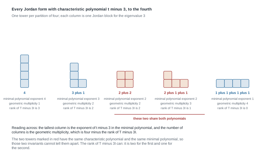
The figure draws each partition as a tower of unit squares, one column per block. The tallest column is the exponent in \(m_T\) and the number of columns is \(\operatorname{geo}(3)\). Rows two and three have the same number of columns and different heights, so \(\operatorname{geo}\) alone does not separate them. Rows three and four have the same height and different numbers of columns, so \(m_T\) alone does not separate them — and since \(p_T\) is the same for all five, \(p_T\) and \(m_T\) together fail on exactly one pair, namely \(2+2\) against \(2+1+1\). What separates them is \(\operatorname{rank}(T - 3I)\), which is \(2\) for the first and \(1\) for the second, equivalently \(\operatorname{geo}(3) = 2\) against \(3\). Week 13 met this pair, as two four-by-four matrices with \(p(t) = (t-2)^4\) and \(m(t) = (t-2)^2\) distinguished by a rank.
Do not over-generalise from the table. In this size the pair \(\big(m_T, \operatorname{geo}(\lambda)\big)\) happens to separate all five classes, because the five ordered pairs in columns two and three are distinct. That is an accident of \(n = 4\). In dimension seven with \(p_T(t) = (t-3)^7\), the partitions \(3+3+1\) and \(3+2+2\) both have \(m_T(t) = (t-3)^3\) and both have \(\operatorname{geo}(3) = 3\); they are separated only further along, by \(\operatorname{rank}(T-3I)^2\), which is \(1+1+0 = 2\) for the first and \(1+0+0 = 1\) for the second. The complete invariant is the whole rank sequence at each eigenvalue, and nothing shorter is guaranteed to work.
The misreading to avoid
The misreading: the Jordan form makes every operator diagonal in disguise — the ones above the diagonal are a bookkeeping artefact, so for any practical purpose I can treat \(T\) as \(\operatorname{diag}(\lambda_1, \dots, \lambda_n)\). The first half misdescribes the theorem and the second half is false in a way that produces wrong numbers.
Take the theorem first. A Jordan matrix is diagonal exactly when every block has size one, and by the counting rule the number of blocks at \(\lambda\) is \(\operatorname{geo}(\lambda)\) while their sizes sum to \(\operatorname{alg}(\lambda)\). So all blocks have size one at \(\lambda\) precisely when \(\operatorname{geo}(\lambda) = \operatorname{alg}(\lambda)\), which is Week 11’s diagonalizability criterion, and it holds at every eigenvalue precisely when \(T\) is diagonalizable. Equivalently, the largest block at each \(\lambda\) has size one precisely when \(m_T\) is a product of distinct linear factors, which is Week 13’s test. The Jordan form does not remove the obstruction to diagonalization; it displays it, as the amount by which the tallest column of each tower exceeds one.
Next, the ones are not removable. If \(J_2(2)\) were similar to \(\operatorname{diag}(2,2) = 2I\), then \(P^{-1}(2I)P = 2I \ne J_2(2)\) for every invertible \(P\), so no such \(P\) exists — a scalar matrix is alone in its similarity class, exactly as Week 13 argued. More sharply, the ranks refuse it: \(\operatorname{rank}(J_2(2) - 2I) = 1\) while \(\operatorname{rank}(2I - 2I) = 0\).
Finally, the numbers. Powers are where the difference shows. Writing \(J_2(2) = 2I + N\) with \(N^2 = 0\), and using that \(I\) and \(N\) commute so the binomial theorem terminates,
\[J_2(2)^{m} = 2^{m}I + m\,2^{m-1}N = \begin{pmatrix} 2^{m} & m\,2^{m-1} \\ 0 & 2^{m} \end{pmatrix} ,\]
against \(\operatorname{diag}(2,2)^{m} = 2^{m}I\). At \(m = 10\) the off-diagonal entry is \(10 \cdot 2^{9} = 5120\), not zero, and it is not a rounding effect: the ratio of the off-diagonal entry to the diagonal one is \(m/2\), which grows without bound. Any long-run estimate made from eigenvalues alone misses a polynomial factor of degree one less than the block size. The general statement, from the same computation on a block of size \(k\), is that the entries of \(J_k(\lambda)^{m}\) are \(\binom{m}{j}\lambda^{m-j}\) along the \(j\)-th superdiagonal.
A quieter version of the misreading is worth naming too: since the block sizes are canonical, so is the basis. They are not the same claim. The multiset of blocks is determined by \(T\); the chain basis realising it is not, as Step 5 showed by exhibiting two of them. What the theorem canonicalises is the matrix, not the change of basis that reaches it.
Practice on your own
These are for your own checking rather than for submission.
- From rank data to a form. Let \(T\) act on \(\mathbb{C}^7\) with \(p_T(t) = (t-5)^7\) and \(\operatorname{rank}(T-5I)^{k} = 7, 4, 2, 1, 0\) for \(k = 0, 1, 2, 3, 4\). Determine the block sizes, write \(J\), and state \(m_T\) and \(\operatorname{geo}(5)\). Then check that the sizes sum to seven and that the largest one matches the index of nilpotency.
- Counting classes. How many similarity classes of \(6 \times 6\) complex matrices have \(p_T(t) = (t-1)^4(t+2)^2\)? Justify the count from the uniqueness theorem, and list the minimal polynomial of each class. Which pairs of classes share both \(p_T\) and \(m_T\)?
- A matrix and its transpose. Prove that every \(A \in M_n(\mathbb{C})\) is similar to \(A^{\mathsf{T}}\). Use that \(\operatorname{rank} M = \operatorname{rank} M^{\mathsf{T}}\) for every matrix, together with \((A^{\mathsf{T}} - \lambda I)^{k} = \big((A - \lambda I)^{k}\big)^{\mathsf{T}}\), and then invoke the classification rather than constructing \(P\).
- The hypothesis you cannot drop. For the quarter-turn rotation \(R\) of \(\mathbb{R}^2\), prove directly that no invertible real \(P\) makes \(P^{-1}RP\) upper triangular, and identify which line of the existence proof fails. Then compute the Jordan form of \(R\) over \(\mathbb{C}\) and the change-of-basis matrix that realises it.
- Nilpotence, three ways. Let \(V\) be finite-dimensional over \(\mathbb{C}\) and \(T \in \mathcal{L}(V)\). Prove the equivalence of: \(T\) is nilpotent; \(p_T(t) = t^{\dim V}\); and every block of the Jordan form of \(T\) carries the eigenvalue \(0\). Then count how many similarity classes of nilpotent operators exist on \(\mathbb{C}^5\).
Where to read more
The three addresses below are offered online at no cost by their providers; availability and licence terms are as those providers state them, and neither is confirmed here.
- MIT OpenCourseWare 18.700 Linear Algebra — a proof-based course whose treatment of generalized eigenvectors and the Jordan form runs parallel to this week, in the same determinant-light style.
- Linear Algebra Done Wrong by Sergei Treil — an abstract-first text that builds the Jordan form from cyclic subspaces and states the classification in the same shape used here.
- MIT OpenCourseWare 18.06 Linear Algebra — the computational complement, useful for practice at ranks of powers and at similarity computations on explicit arrays.
- The optional Roman alignment for this week is the chapter on eigenvalues and eigenvectors, in the section on the Jordan canonical form. That text is an optional reference: a borrowed or library copy suffices, purchase is never required, and nothing from it is reproduced here.
- Course pages: the notes overview, the syllabus, the schedule, and the resources page. The learning management system remains authoritative for section logistics and graded details.
Where this goes next
These notes end here, so read the term backwards instead. Week 1 gave you a set with eight axioms and a field acting on it, and the interesting question was never what a vector is but how a subspace sits inside its parent. Week 2 measured the objects and proved the measurement well defined. Weeks 3 and 4 turned attention to the maps and showed that a matrix is what a map looks like after somebody chose a basis — leaving the question of which features belong to the map. Weeks 5 through 9 added one piece of structure, an inner product, and got length, angle, orthonormal bases, projections, and the adjoint out of it. Weeks 10 through 12 asked which operators are as simple as a diagonal matrix, and found that self-adjointness guarantees it. Week 13 settled for triangular when diagonal was unavailable and introduced the polynomial that decides. Week 14 enlarged the eigenspaces until they filled the space and broke the leftover into chains. This week named the result and proved it complete.
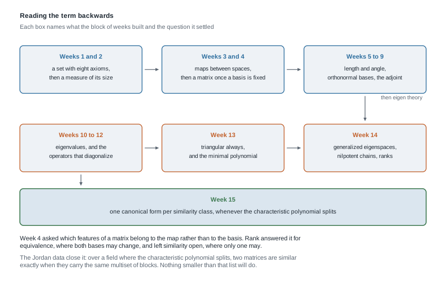
The figure lays that sequence out in one picture, with the Week 4 question at the start of the lower bar and its resolution at the end: the term was one argument rather than four topics, each block supplying the tool the next block spent. The inner-product weeks look like a detour and are not one — Week 12’s spectral theorem makes the well-behaved case easy, and Week 13’s Schur theorem makes Cayley-Hamilton honest.
Three directions open from here. The singular value decomposition factors any matrix, rectangular included, using two orthonormal bases rather than one; it is the stable relative of the eigenvalue decomposition, and the one that survives contact with measured data. The general setting for canonical forms is modules over a principal ideal domain: a vector space with an operator is exactly a module over the polynomial ring \(F[t]\), and the structure theorem for finitely generated modules over such a ring specialises to the Jordan form when \(p_T\) splits and to the rational canonical form when it does not. Dropping finite-dimensionality changes the subject entirely — spectra replace eigenvalue lists, and operators can have no eigenvectors at all. To look back, Week 14 carries the generalized eigenspaces and chains this page assembled, Week 13 the minimal polynomial, and Week 4 the similarity question that started it; the notes index and the course home page list everything here.