Week 13 — Interval estimation and the shape of uncertainty
Where this week starts
Week 12 left you holding a point estimate and a number beside it. The maximum likelihood estimator \(\hat\theta\) is asymptotically normal, its variance is approximately \(1/(n I_1(\theta))\), and you can estimate that variance from the observed information at the maximum. So you can write \(\hat\theta \pm 1.96\,\mathrm{se}(\hat\theta)\) and stop. Almost everyone does stop there, and almost everyone who stops there believes the resulting pair of numbers means something it does not.
This week takes the step from a standard error to an interval seriously, because the step is not one argument but several, and they do not always land in the same place. Three machines are already in your hands. Week 4 built the pivotal interval: find a function of data and parameter whose distribution is free of the parameter, then invert an exact probability statement into a set of parameter values. Week 12 built the Wald interval without quite naming it: take the asymptotic normality of \(\hat\theta\) at face value and step out symmetrically. Week 9 built the credible interval: put a prior on \(\theta\), compute the posterior, and cut off the middle 95 percent of it. A fourth machine, the bootstrap, is coming in the next course, and it is worth previewing here because it makes the shape question unavoidable.
Take one data set — three successes in twenty trials, say — and run all of them. You will get four intervals that are not the same. One of them will contain negative values of a probability. Two of them will be visibly lopsided in opposite directions from a third. Nothing has gone wrong. Each machine is answering a different question, and this week is about learning to hear the difference.
By Thursday you should be able to compute a Wald interval, a likelihood-ratio interval and a posterior interval on the same model, say precisely what each one claims, predict from the shape of the log-likelihood which way they will disagree, and diagnose which of them has actually failed when one of them has.
Why this matters downstream
Here is the stake, and it is not hypothetical arithmetic. A reliability group observes three failures in twenty units and reports the Wald interval for the failure probability. The lower endpoint comes out at \(-0.006\), so they truncate it at zero and report “zero to 0.306, 95 percent confidence”. The truncation looks like tidiness. It is not: at a true failure probability of \(0.15\) the recipe they used covers the truth 81.9 percent of the time, not 95, and near the boundary it collapses further. An interval that claims a coverage it does not have is worse than a point estimate with no interval, because it launders a guess into a guarantee.
The forward stake is just as concrete. Week 14 asks what any of this is worth when the model is wrong, and that question is unanswerable until you can say what an interval claims when the model is right. Regression, generalized linear models, and every survival analysis you will ever read report likelihood-based intervals by default; the profile-likelihood machinery below is the whole reason those intervals are not symmetric.
What you will be able to do
- Derive the Wald and likelihood-ratio intervals from the same Taylor expansion, and state exactly which approximation separates them.
- Compute all three interval types for a binomial sample by hand and by machine, and compare them on one parameter axis.
- Explain what a coverage probability is a statement about, what a posterior probability is a statement about, and why interchanging the two is a category error rather than a rounding error.
- Predict, from the curvature and skew of a log-likelihood, which interval will be widest and in which direction.
- Diagnose a failing interval procedure by computing its exact coverage, rather than trusting the level printed on it.
- Describe how a bootstrap percentile interval is built, and name what the next course has to add before it can be trusted.
Words worth owning
| Term | What it means in this course |
|---|---|
| Confidence interval | A random set produced by a rule whose coverage is at least the stated level. The level belongs to the rule, never to a realized pair of numbers. |
| Coverage probability | \(P_\theta(\theta \in C(X))\): the probability over repeated samples, with \(\theta\) held fixed, that the set the rule produces contains it. |
| Wald interval | \(\hat\theta \pm z_{1-\alpha/2}\,\mathrm{se}(\hat\theta)\). Equivalently, the likelihood interval computed on a quadratic stand-in for the log-likelihood. |
| Deviance | \(D(\theta) = 2[\ell(\hat\theta) - \ell(\theta)]\), twice the drop in the log-likelihood below its maximum. A distance measured in likelihood units. |
| Likelihood-ratio interval | The set of \(\theta\) whose deviance stays below a calibrated cut, usually \(\chi^2_{1, 1-\alpha}\). |
| Profile likelihood | What is left of the likelihood in the parameter you care about once the others have been maximized out at each of its values. |
| Credible interval | An interval carrying stated posterior probability. A statement about \(\theta\) given these data and this model, not about repetition. |
| Bootstrap percentile interval | Endpoints read off the percentiles of the estimate’s distribution across resamples of the observed data. |
Three machines, one parameter axis
Fix notation for the whole section. Let \(X_1, \dots, X_n\) be independent with density or mass function \(f(x \mid \theta)\) for a scalar \(\theta\) in an open parameter space \(\Theta\), write \(\ell(\theta) = \sum_{i=1}^n \log f(X_i \mid \theta)\) for the log-likelihood, and let \(\hat\theta\) maximize it. Write \(\alpha = 0.05\) throughout, so \(z_{0.975} = 1.95996\) and \(\chi^2_{1, 0.95} = 3.84146\).
The pivot when you can get one
The cleanest machine is Week 4’s. A pivotal quantity is a function \(Q(X, \theta)\) whose distribution is the same under every \(\theta \in \Theta\). Choose \(a\) and \(b\) with \(P_\theta(a \le Q(X, \theta) \le b) = 1 - \alpha\) — possible precisely because the law of \(Q\) does not move — and define \(C(X) = \{\theta : a \le Q(X, \theta) \le b\}\). For each fixed \(\theta\) the events \(\{\theta \in C(X)\}\) and \(\{a \le Q(X, \theta) \le b\}\) are the same set of samples written twice, so the coverage is exactly \(1 - \alpha\) at every \(\theta\). No limit, no approximation, no appeal to large \(n\).
The trouble is availability. Exact pivots live in a small neighbourhood of models: normal theory gives \((\bar{X} - \mu)/(S/\sqrt{n}) \sim t_{n-1}\) and \((n-1)S^2/\sigma^2 \sim \chi^2_{n-1}\); the exponential gives \(2\lambda \sum_i X_i \sim \chi^2_{2n}\); the uniform on \((0, \theta)\) gives \(X_{(n)}/\theta\) with distribution function \(u^n\). Step outside and there is usually nothing exact to invert. For the binomial there is no pivot at all, because the data are discrete and no function of \((X, p)\) can have a distribution free of \(p\). That is not a temporary gap in the theory; it is a structural fact about discrete models, and it is why the rest of this page exists.
The two intervals the likelihood gives
Expand the log-likelihood about its maximum. Because \(\ell'(\hat\theta) = 0\) at an interior maximum, the linear term vanishes and
\[\ell(\theta) \approx \ell(\hat\theta) - \tfrac{1}{2} J(\hat\theta)\,(\theta - \hat\theta)^2, \qquad J(\hat\theta) = -\ell''(\hat\theta),\]
where \(J\) is the observed information from Week 12. Multiply the drop by two:
\[D(\theta) = 2\big[\ell(\hat\theta) - \ell(\theta)\big] \approx J(\hat\theta)\,(\hat\theta - \theta)^2.\]
Now read the same approximate identity in two directions, and the two frequentist machines fall out of it.
Read it from right to left. Week 12 gives \(\sqrt{n}(\hat\theta - \theta) \xrightarrow{d} N(0, 1/I_1(\theta))\) and \(J(\hat\theta)/n \to I_1(\theta)\) in probability, so \(\sqrt{J(\hat\theta)}(\hat\theta - \theta)\) converges in distribution to a standard normal by Slutsky. Collecting the values of \(\theta\) for which that standardized quantity is at most \(z_{1-\alpha/2}\) in absolute value gives
\[\hat\theta \pm z_{1-\alpha/2}\,\mathrm{se}(\hat\theta), \qquad \mathrm{se}(\hat\theta) = J(\hat\theta)^{-1/2},\]
the Wald interval. Read it from left to right instead. Squaring a standard normal gives a \(\chi^2_1\) variable, so under the same conditions \(D(\theta_0) \xrightarrow{d} \chi^2_1\) at the true \(\theta_0\) — this is Wilks’ theorem — and the set
\[C_{\mathrm{LR}}(X) = \big\{\theta \in \Theta : D(\theta) \le \chi^2_{1, 1-\alpha}\big\}\]
is the likelihood-ratio interval. Its asymptotic coverage is \(1 - \alpha\) for the same reason the Wald interval’s is.
Wilks’ theorem needs the Week 7 regularity conditions and needs them all: the true value interior to \(\Theta\), a common support not depending on \(\theta\), a log-likelihood twice differentiable in \(\theta\), an information \(I_1(\theta)\) finite and strictly positive, and enough smoothness to differentiate under the integral sign. Every one of them is checkable in a given model, and the uniform on \((0, \theta)\) fails the second, and with it the third and fifth. Check before you cut.
So the two frequentist intervals are the same cut taken on two different curves: the Wald interval cuts the parabola, the likelihood-ratio interval cuts the log-likelihood itself. They coincide exactly when the log-likelihood is exactly quadratic, which happens for a normal mean with known variance and essentially nowhere else. Everywhere else they differ by however much the real curve departs from its parabola, and that departure is the shape information the Wald interval throws away.
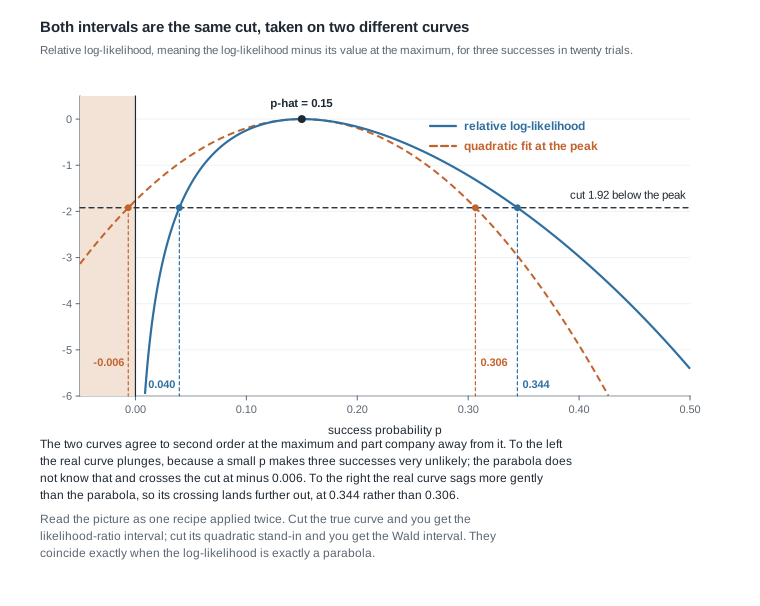
The figure draws both curves for three successes in twenty trials. To the left of the maximum the true curve plunges toward minus infinity as \(p\) approaches zero, because three successes are impossible at \(p = 0\); the parabola knows nothing about that and wanders across the boundary. To the right the true curve sags more gently than the parabola, so its crossing lands further out. The result is an asymmetric likelihood-ratio interval sitting entirely inside \((0,1)\) and a symmetric Wald interval that does not.
One consequence deserves its own sentence, because it decides which machine to trust in practice. The likelihood-ratio interval is equivariant under any monotone reparameterization. If \(\phi = g(\theta)\) with \(g\) strictly increasing, then \(\hat\phi = g(\hat\theta)\), the deviance in \(\phi\) at \(g(\theta)\) equals the deviance in \(\theta\) at \(\theta\), and so the interval for \(\phi\) is exactly the image under \(g\) of the interval for \(\theta\). The Wald interval has no such property: the standard error transforms by the delta method as \(|g'(\hat\theta)|\,\mathrm{se}(\hat\theta)\), and stepping out symmetrically in \(\phi\) is not the image of stepping out symmetrically in \(\theta\). The second worked example builds three different Wald intervals for one variance to make that concrete.
The posterior interval and what it asserts
The third machine changes what kind of object \(\theta\) is. Give it a prior density \(\pi(\theta)\) and Bayes’ theorem returns the posterior
\[\pi(\theta \mid x) = \frac{L(\theta)\,\pi(\theta)}{\int_\Theta L(t)\,\pi(t)\,dt},\]
a genuine probability distribution over the parameter space. A \(1 - \alpha\) credible interval is any set carrying posterior probability \(1 - \alpha\); the equal-tailed choice takes the \(\alpha/2\) and \(1 - \alpha/2\) posterior quantiles, and the highest-posterior-density choice takes the shortest such set. The sentence “the probability that \(\theta\) lies between these numbers is 0.95” is legitimate here and nowhere else in this course, and the words “within this model and under this prior” are part of the claim, not a disclaimer bolted onto it.
Two structural remarks. First, a credible interval respects the boundary automatically: the posterior puts no mass outside \(\Theta\), so no quantile of it can land outside \(\Theta\). Second, the equal-tailed version is equivariant like the likelihood-ratio interval, because posterior quantiles ride along under a monotone change of variables even though the density does not. The highest-posterior-density version is the exception, and the reason sits in that last clause: under \(\phi = g(\theta)\) the density acquires a Jacobian factor, so the shortest set in \(\phi\) is not in general the image of the shortest set in \(\theta\) unless \(g\) is affine. Together they explain most of what you will see when the intervals are drawn side by side.
Where the three agree and where they part
The regime of agreement
Suppose the log-likelihood is close to quadratic near its maximum, the prior is flat over the range where the likelihood is appreciable, and \(n\) is large. Then all three machines return nearly the same interval, and the reason is that all three are reading the same curve. The Wald interval cuts the parabola. The likelihood-ratio interval cuts a curve that is nearly that parabola. The posterior is proportional to \(L(\theta)\) times a nearly constant prior, so it is nearly a normal density centred at \(\hat\theta\) with variance \(1/J(\hat\theta)\) — this is the Bernstein-von Mises phenomenon, and it is the precise sense in which a flat-prior Bayesian and a likelihood frequentist stop disagreeing in large samples. Numerically, the same three successes in twenty trials scaled up to thirty successes in two hundred give a Wald interval of \((0.1005, 0.1995)\), a likelihood-ratio interval of \((0.1051, 0.2038)\), and a flat-prior posterior interval of \((0.1073, 0.2062)\). All three have width \(0.099\) to three decimal places, and no endpoint differs from another by more than \(0.007\).
Agreement in the regime is not agreement in meaning. The three sentences attached to those nearly identical numbers remain different sentences: a statement about repeated sampling, a statement about where the likelihood is not much lower than its peak, and a statement about posterior probability. When they coincide numerically, you should say so and move on; when they do not, the gap is the information.
Four ways the agreement breaks
Small \(n\). The quadratic approximation is an \(n \to \infty\) statement, and at \(n = 20\) near a boundary it is simply false. Everything in the first worked example is this failure.
A boundary. When \(\hat\theta\) sits near the edge of \(\Theta\), the Wald interval crosses it and the Wilks calibration itself begins to drift. When \(\hat\theta\) sits on the edge, the theorem does not apply at all.
Skew in the likelihood. A log-likelihood that falls away faster on one side than the other produces an asymmetric likelihood-ratio interval, and the Wald interval — symmetric by construction — cannot reproduce it. Rate parameters, variance components and odds ratios are all like this.
An informative prior. Where the prior is not flat over the range the likelihood cares about, the posterior interval moves, and it should. That movement is a modelling choice, and it must be reported as one.
The first of these is measurable. Coverage is a computable property of a rule, and here it can be computed exactly rather than simulated: for each \(x\) from zero to twenty, decide whether the interval the rule builds from \(x\) contains a candidate \(p\), and add up the binomial probabilities of the values of \(x\) for which it does.
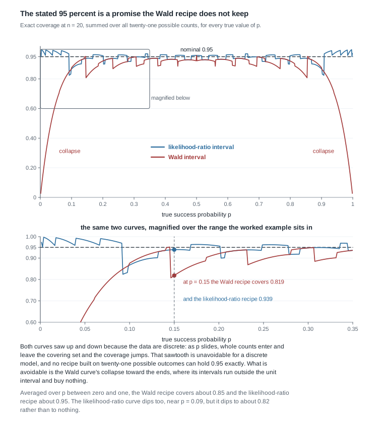
Read the figure carefully, because it teaches two separate things. The sawtooth in both curves is unavoidable: the data are discrete, so as \(p\) slides continuously, whole outcomes enter and leave the covering set and the coverage jumps. No rule built on twenty-one possible outcomes holds exactly 0.95 at every \(p\), and the honest description of any of them is “at least approximately 95 percent, with excursions”. What is avoidable is the collapse of the Wald curve toward the ends, where its coverage falls past 0.80, past 0.50, and finally to nothing. Averaged across \(p\), the Wald recipe covers about 0.85 against the likelihood-ratio recipe’s 0.95. At \(p = 0.15\) the two differ by twelve parts in a hundred, which is the entire gap between an interval worth reporting and one worth withdrawing.
The bootstrap, previewed honestly
There is a fourth machine, and it dispenses with the likelihood altogether. Treat the observed sample as a stand-in for the population; draw \(B\) resamples of size \(n\) from it with replacement; recompute the estimator on each; and read the \(2.5\) and \(97.5\) percentiles off the resulting collection. That is the bootstrap percentile interval, and its appeal is obvious: no pivot, no derivative, no prior, no closed form for the sampling distribution of anything.
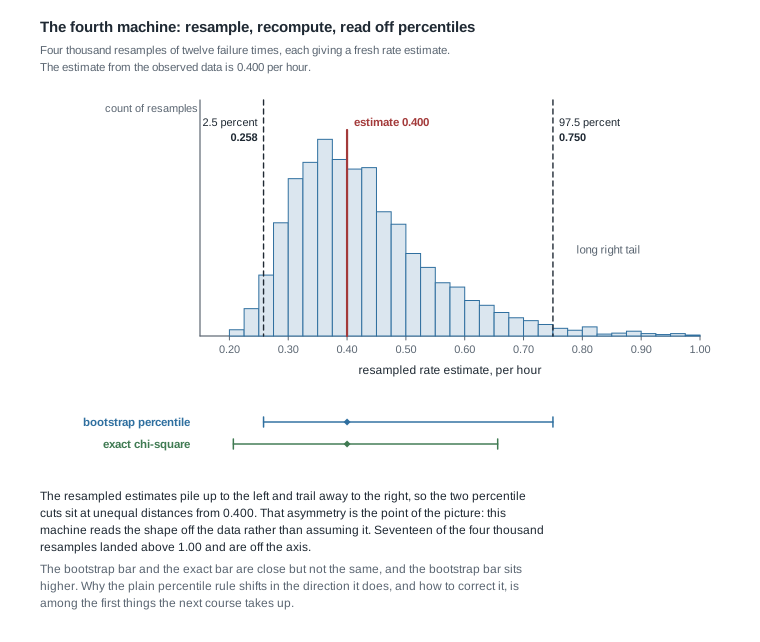
The figure resamples twelve failure times whose total is thirty hours, so the rate estimate from the observed data is \(\hat\lambda = 12/30 = 0.400\) per hour. The resampled estimates pile up on the left and trail away on the right, exactly as the shape of the likelihood for a rate predicts, and the two percentile cuts sit at unequal distances from \(0.400\). That is the machine’s real selling point: it reads the shape off the data instead of assuming it.
It is also where the honesty is required. The bootstrap bar in the figure runs from \(0.258\) to \(0.750\), while the exact chi-square interval for these data runs from \(0.207\) to \(0.656\). The bootstrap bar is shifted upward, and not by accident: the percentile rule uses the spread of \(\hat\lambda^*\) around \(\hat\lambda\) as a stand-in for the spread of \(\hat\lambda\) around \(\lambda\), and when the sampling distribution is skewed those two are not mirror images. Correcting for that — the bias-corrected and accelerated variants, the bootstrap-\(t\), and the theory that says when any of it is consistent — is Mathematical Statistics II’s material, not this week’s. Take the picture as a statement about shape and a promissory note, not as a fourth interval you may report today.
Worked example — three intervals for three successes in twenty trials
Setting. A laboratory tests twenty independently manufactured seals under an accelerated protocol and records three failures. Model the failures as \(X \sim \mathrm{Binomial}(n = 20, p)\) with \(x = 3\) observed. The estimand is \(p\), the failure probability of a seal under this protocol. Take \(\alpha = 0.05\).
Step one, the estimate and the curve. The log-likelihood, dropping the binomial coefficient because it does not involve \(p\), is \(\ell(p) = 3\log p + 17 \log(1 - p)\). Differentiating, \(\ell'(p) = 3/p - 17/(1-p)\), which vanishes at \(p = 3/20 = 0.15\), so \(\hat p = 0.15\). Differentiating again, \(\ell''(p) = -3/p^2 - 17/(1-p)^2\), and at \(\hat p\) this is \(-3/0.0225 - 17/0.7225 = -133.333 - 23.529 = -156.863\). So \(J(\hat p) = 156.863\), which is the familiar \(n/\{\hat p(1 - \hat p)\} = 20/0.1275\).
Step two, the Wald interval. The standard error is \(\mathrm{se}(\hat p) = J(\hat p)^{-1/2} = \sqrt{0.1275/20} = \sqrt{0.006375} = 0.079844\). The half-width is \(1.95996 \times 0.079844 = 0.156491\), so the interval runs from \(0.15 - 0.156491 = -0.006491\) to \(0.15 + 0.156491 = 0.306491\).
Step three, the likelihood-ratio interval. At the maximum, \(\ell(\hat p) = 3\log 0.15 + 17\log 0.85 = 3(-1.897120) + 17(-0.162519) = -8.454182\). The cut sits half of \(3.84146\) below that, at \(-8.454182 - 1.920729 = -10.374911\), so the endpoints are the two roots of
\[3\log p + 17 \log(1 - p) = -10.374911.\]
This is not solvable in closed form; bisection on each side of \(\hat p\) settles it. The lower root is \(p = 0.039579\) and the upper root is \(p = 0.344376\). Check the lower one by substitution: \(3\log(0.039579) = 3(-3.2294566) = -9.6883698\) and \(17\log(0.960421) = 17(-0.0403835) = -0.6865195\), and the two sum to \(-10.3748893\), within two parts in a hundred thousand of the target.
Step four, the posterior interval. With a \(\mathrm{Beta}(a, b)\) prior the posterior is \(\mathrm{Beta}(a + x,\, b + n - x)\), the conjugate update from Week 9. A flat \(\mathrm{Beta}(1,1)\) prior gives \(\mathrm{Beta}(4, 18)\), whose posterior mean is \(4/22 = 0.1818\) and whose equal-tailed 95 percent interval is \((0.0545, 0.3634)\). The Jeffreys prior \(\mathrm{Beta}(1/2, 1/2)\) gives \(\mathrm{Beta}(3.5, 17.5)\), posterior mean \(3.5/21 = 0.1667\), and interval \((0.0441, 0.3486)\).
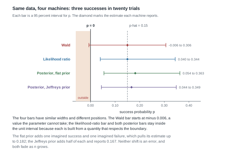
What the picture shows. The four bars have similar widths and different positions. The Wald bar is the only one that leaves the parameter space, and it does so because it was built from a parabola that has no idea \(p\) cannot be negative. The likelihood-ratio bar is shifted right of the Wald bar at both ends, reflecting the right skew of the likelihood. The two posterior bars sit slightly right again, because a flat prior on \((0,1)\) is not neutral about a small \(p\): adding one imagined success and one imagined failure moves the estimate from \(0.15\) up to \(0.182\), and the Jeffreys prior, adding half of each, moves it to \(0.167\). None of these shifts is an error. Each is a different, statable claim.
What it assumed. Independence across the twenty seals, a constant failure probability, and — for the last two bars — a prior you would be willing to defend before seeing the data. The first two assumptions are the ones a manufacturing process most often breaks, through a shared batch of material.
The same reasoning, transferred
Change the model and keep the structure. Twelve units are run to failure and the times, in hours, are \(0.2, 0.3, 0.6, 0.9, 1.2, 1.5, 2.0, 2.4, 3.3, 4.1, 5.8, 7.7\), which total exactly \(30.0\). Model them as independent \(\mathrm{Exponential}(\lambda)\) with density \(\lambda e^{-\lambda x}\) for \(x \gt 0\), so the estimand \(\lambda\) is a failure rate per hour. Then \(\ell(\lambda) = 12 \log \lambda - 30\lambda\), so \(\hat\lambda = 12/30 = 0.400\) per hour, and \(J(\hat\lambda) = 12/\hat\lambda^2 = 75\), giving \(\mathrm{se}(\hat\lambda) = 1/\sqrt{75} = 0.11547\).
The three machines run again. The Wald interval is \(0.400 \pm 1.95996 \times 0.11547\), that is \((0.1737, 0.6263)\). The deviance simplifies to \(D(\lambda) = 24[u - 1 - \log u]\) with \(u = \lambda/\hat\lambda\), and setting it equal to \(3.84146\) gives \(u = 0.5355\) and \(u = 1.6772\), so the likelihood-ratio interval is \((0.2142, 0.6709)\). Here, unusually, an exact pivot also exists: \(\sum_i X_i\) is \(\mathrm{Gamma}(12, \lambda)\), so \(2\lambda \sum_i X_i \sim \chi^2_{24}\) whatever \(\lambda\) is, and inverting \(12.4012 \le 60\lambda \le 39.3641\) gives the exact interval \((0.2067, 0.6561)\).
What stayed the same: one curve, one cut, and one symmetric step. What changed: the exact pivot is available, so the two approximations can be graded rather than merely compared. The likelihood-ratio interval is close to exact at both ends; the Wald interval is too low at both ends, by \(0.033\) at the bottom and \(0.030\) at the top, because it insists on symmetry that the rate likelihood does not have. One more thing changed, and it is worth noticing: with the Jeffreys prior \(\pi(\lambda) \propto 1/\lambda\) the posterior is \(\mathrm{Gamma}(12,\, 30)\), under which \(2\lambda \sum_i x_i\) again has the \(\chi^2_{24}\) distribution — so the credible interval is numerically identical to the exact confidence interval, \((0.2067, 0.6561)\). Same numbers, two different sentences.
A computation you can run
Derive, compute, critique. Every number above is reproducible in a few lines of R, and typing them is the fastest route to believing the figure.
x <- 3; n <- 20; phat <- x / n

# Wald
phat + c(-1, 1) * qnorm(0.975) * sqrt(phat * (1 - phat) / n)   # -0.0065  0.3065

# likelihood ratio: cut the deviance at qchisq(0.95, 1)
dev <- function(p) 2 * (dbinom(x, n, phat, log = TRUE) - dbinom(x, n, p, log = TRUE))
cut <- qchisq(0.95, 1)
c(uniroot(function(p) dev(p) - cut, c(1e-10, phat))$root,
  uniroot(function(p) dev(p) - cut, c(phat, 1 - 1e-10))$root)  #  0.0396  0.3444

# posterior with a flat prior, then with the Jeffreys prior
qbeta(c(0.025, 0.975), x + 1,   n - x + 1)                     #  0.0545  0.3634
qbeta(c(0.025, 0.975), x + 0.5, n - x + 0.5)                   #  0.0441  0.3486
Coverage is computable too, by exactly that enumeration.
cover <- function(p, n = 20) {
  x  <- 0:n
  ph <- x / n
  se <- sqrt(ph * (1 - ph) / n)
  lo <- ph - qnorm(0.975) * se
  hi <- ph + qnorm(0.975) * se
  sum(dbinom(x, n, p)[lo <= p & p <= hi])
}
cover(0.15)   # 0.8185
cover(0.05)   # 0.6389
Two habits are being modelled here: a claimed coverage is a checkable claim, so check it; and exact enumeration beats simulation whenever the sample space is small enough to walk, because it removes Monte Carlo noise from the verdict.
Second worked example — an interval for a normal variance
Setting. Week 4 weighed a reference mass eight times on one balance and recorded, in grams, \(10.2, 9.8, 10.5, 10.1, 9.6, 10.4, 9.9, 10.3\). The mean is \(\bar{x} = 80.8/8 = 10.1\) and the residual sum of squares is \(\sum_i (x_i - \bar{x})^2 = 0.68\), so \(s^2 = 0.68/7 = 0.097143\). Model the readings as independent \(N(\mu, \sigma^2)\) with both parameters unknown, and take the estimand to be \(\sigma^2\), the balance’s repeatability variance. This example strains a condition the first one did not: there are two parameters, and \(n\) is small.
Step one, profile out the nuisance parameter. For fixed \(\sigma^2\) the log-likelihood is maximized over \(\mu\) at \(\bar{x}\), so the profile log-likelihood is
\[\ell_p(\sigma^2) = -\frac{n}{2}\log(2\pi) - \frac{n}{2}\log \sigma^2 - \frac{SS}{2\sigma^2}, \qquad SS = \sum_{i=1}^n (x_i - \bar{x})^2 = 0.68 .\]
Setting the derivative to zero gives \(-n/(2\sigma^2) + SS/(2\sigma^4) = 0\), so \(\hat\sigma^2 = SS/n = 0.68/8 = 0.085\). Note that this is the maximum likelihood estimate, with divisor \(n\), and not the unbiased \(s^2 = 0.097143\) with divisor \(n - 1\).
Step two, the exact pivotal interval. From Week 4, \(SS/\sigma^2 \sim \chi^2_{n-1} = \chi^2_7\) whatever \(\mu\) and \(\sigma^2\) are. The equal-tailed cuts are \(1.68987\) and \(16.01276\), and inverting \(1.68987 \le 0.68/\sigma^2 \le 16.01276\) — legitimate because all three quantities are positive, so taking reciprocals reverses both inequalities — gives
\[\frac{0.68}{16.01276} \le \sigma^2 \le \frac{0.68}{1.68987}, \qquad \text{that is} \qquad 0.04247 \le \sigma^2 \le 0.40240 .\]
Step three, the likelihood-ratio interval. Write \(r = \sigma^2/\hat\sigma^2\). Substituting into the profile log-likelihood and cancelling the constants,
\[D(\sigma^2) = 2\big[\ell_p(\hat\sigma^2) - \ell_p(\sigma^2)\big] = n\Big[\log r + \frac{1}{r} - 1\Big],\]
because \(SS/\hat\sigma^2 = n\) exactly. That function is zero at \(r = 1\) and increases in both directions, as it must. Setting \(8[\log r + 1/r - 1] = 3.84146\) gives \(r = 0.43046\) and \(r = 3.22113\), so the interval is \((0.43046 \times 0.085,\; 3.22113 \times 0.085) = (0.03659, 0.27380)\).
Step four, the Wald intervals, plural. Differentiating the profile twice gives \(\ell_p''(\sigma^2) = n/(2\sigma^4) - SS/\sigma^6\), which at \(\hat\sigma^2\) equals \(-n/(2\hat\sigma^4)\), so \(\mathrm{se}(\hat\sigma^2) = \hat\sigma^2\sqrt{2/n} = 0.085 \times 0.5 = 0.0425\). The Wald interval for \(\sigma^2\) is therefore \(0.085 \pm 1.95996 \times 0.0425 = (0.00170, 0.16830)\). Now redo it on the log scale. By the delta method \(\mathrm{se}(\log \hat\sigma^2) = \sqrt{2/n} = 0.5\), and \(\log 0.085 = -2.46510\), so the interval for \(\log\sigma^2\) is \((-3.44508, -1.48512)\); exponentiating gives \((0.03190, 0.22648)\) for \(\sigma^2\).
| Machine | Interval for \(\sigma^2\) | Width |
|---|---|---|
| Exact pivotal, from \(\chi^2_7\) | \((0.04247,\ 0.40240)\) | \(0.35993\) |
| Likelihood ratio | \((0.03659,\ 0.27380)\) | \(0.23721\) |
| Wald on the variance scale | \((0.00170,\ 0.16830)\) | \(0.16660\) |
| Wald on the log-variance scale | \((0.03190,\ 0.22648)\) | \(0.19458\) |
| Posterior, reference prior | \((0.04247,\ 0.40240)\) | \(0.35993\) |
Reading the table. Four rows are four different claims about one number, and the spread between them at \(n = 8\) is the whole lesson. The exact row is the standard against which the others are graded, because for this model an exact pivot genuinely exists. Both approximations are too short and both are shifted low, the Wald far more than the likelihood ratio, and the reason is visible in the profile: the log-likelihood in \(\sigma^2\) is strongly right-skewed at this sample size, so a symmetric step badly understates how large \(\sigma^2\) might be. Reparameterizing to \(\log \sigma^2\) helps a great deal, moving the lower endpoint from \(0.0017\) to \(0.0319\) — but “helps a great deal” is not “is correct”, and the fact that the same machine produces two different intervals for one estimand is the non-equivariance of the previous section, in numbers.
The last row deserves a comment. Under the standard reference prior \(\pi(\mu, \sigma^2) \propto 1/\sigma^2\), the marginal posterior of \(\sigma^2\) is inverse-gamma with shape \((n-1)/2\) and scale \(SS/2\), which is the same as saying \(SS/\sigma^2\) has the \(\chi^2_7\) distribution given the data. The posterior quantiles therefore reproduce the exact confidence interval digit for digit. That is a real and useful fact about this model and this prior, and it is also a coincidence you must not generalize: for the binomial no prior can achieve it, because coverage there jumps as \(p\) moves — the sawtooth two sections above — while a nominal level is a constant, and a function with jumps cannot equal a constant. Read the agreement as “these two sentences happen to pick out the same set here”, not as “the two frameworks agree”.
The misreading to avoid
Here is the sentence that arrives every year, once the table above is on the board:
“The four machines gave four different intervals for the same data, so three of them must be wrong. Tell me which one is right.”
The request is reasonable and the premise is not. Start with what would actually make an interval wrong: a rule is wrong when it does not deliver what it claims. A confidence interval claims coverage, so its correctness is settled by computing coverage, which the enumeration above does. A credible interval claims posterior probability under a stated prior, so its correctness is settled by checking the posterior arithmetic. Those are different audits, and passing one says nothing about the other. Two rules can both pass their own audit and still return different numbers, because they were never promising the same thing.
By that standard, exactly one row of the first worked example fails: the Wald interval, whose stated coverage is \(0.95\) and whose actual coverage at \(p = 0.15\) is \(0.819\). It is not wrong because it disagrees with the others. It is wrong because it disagrees with itself. The likelihood-ratio interval and both posterior intervals disagree with each other just as loudly and all three survive their audits.
Then the second half of the reply, which is the part worth keeping. Disagreement is a measurement. When the Wald and likelihood-ratio intervals differ, the size of the difference is a direct read-out of how far the log-likelihood is from quadratic, which is a read-out of how little the asymptotics have taken hold at this \(n\). When the two posterior intervals differ from each other, the difference measures the prior’s influence, and it shrinks as the data accumulate. When all of them coincide, as they nearly did at two hundred trials, you have learned that you are in the regime where the choice does not matter. Treating the spread as noise to be argued away discards all of that.
One counterexample to finish, because it shows that even the likelihood machine needs its calibration checked rather than assumed. Take \(X_1, \dots, X_n\) uniform on \((0, \theta)\) with \(M = X_{(n)}\). The likelihood is \(\theta^{-n}\) for \(\theta \ge M\) and zero below, so \(\hat\theta = M\) and, for \(\theta \ge M\),
\[D(\theta) = 2\big[\ell(M) - \ell(\theta)\big] = 2n \log(\theta/M).\]
Its exact distribution follows from \(P_\theta(M/\theta \le u) = u^n\) on \((0,1)\):
\[P_\theta\big(D(\theta) \gt w\big) = P_\theta\!\left(\frac{M}{\theta} \lt e^{-w/(2n)}\right) = e^{-w/2},\]
so \(D(\theta)\) is exponential with mean two — that is, exactly \(\chi^2_2\), at every \(n\), with no limit taken. Cut it at \(\chi^2_{1,0.95} = 3.84146\) as Wilks would have you do and the coverage is \(1 - e^{-1.920729} = 0.8535\), never improving with more data. Cut it at \(\chi^2_{2,0.95} = 5.99146\) instead and you get \(\theta \le M e^{2.99573/n}\) with coverage exactly \(0.95\) — which is precisely Week 4’s uniform pivot \(M/\theta\) inverted one-sidedly rather than equal-tailed, since \(-\log(0.05) = 2.99573\). The machinery was fine; the calibration was borrowed from a theorem whose conditions this model fails. Name them exactly: the support moves with \(\theta\), so the likelihood jumps at \(\theta = M\) instead of curving there, and the maximizer sits at the edge of the region where the likelihood is positive. What does not fail is the condition students reach for first: the true \(\theta_0\) is interior to \(\Theta = (0, \infty)\). State the assumption, check the special case: the audit habit is not decoration here, it is the difference between 85 percent and 95.
Practice on your own
A third model, three machines. For a Poisson sample with \(n = 10\) and \(\bar{x} = 0.5\), derive \(\hat\lambda\), the observed information, the Wald interval, and the deviance function \(D(\lambda)\) in closed form. Compute the likelihood-ratio interval numerically and the gamma posterior interval under \(\pi(\lambda) \propto \lambda^{-1/2}\). Rank the three by width and explain the ranking from the shape of \(\ell\).
A counterexample hunt. Find the smallest \(n\) and a count \(x\) for which the Wald interval for a binomial proportion has an upper endpoint exceeding one. Then show that the likelihood-ratio interval can never leave \([0,1]\), using only the fact that \(\ell(p) \to -\infty\) at each endpoint when \(0 \lt x \lt n\).
An audit. A colleague writes: “Week 4 gave the interval \((0.206, 0.634)\) for \(\sigma\). Squaring the endpoints gives \((0.042, 0.402)\) for \(\sigma^2\), which is exactly the chi-square interval on that scale. So I can equally square the endpoints of a Wald interval for \(\sigma\) to get the Wald interval for \(\sigma^2\).” Coverage is not what separates these two moves: for nonnegative endpoints \(L\) and \(U\), the events \(\{\sigma \in (L, U)\}\) and \(\{\sigma^2 \in (L^2, U^2)\}\) coincide, since squaring is increasing on the positive half-line, so both transformed intervals carry the coverage of their originals. Only one move, though, reproduces what the machine itself builds on the new scale. Identify which, name the property that licenses it, then compute the Wald interval for \(\sigma\) from the second worked example, square it, and set it beside the \((0.00170, 0.16830)\) in the table.
A simulation to describe. Predict, before running anything, whether the flat-prior credible interval for a binomial proportion over-covers or under-covers in the frequentist sense at \(p = 0.05\) and \(n = 20\). Write out the enumeration that would settle it, name the quantity you would report, and say what result would falsify your prediction.
A fourth machine you can derive. The score interval inverts \((\hat p - p)/\sqrt{p(1-p)/n}\) — note the denominator uses the candidate \(p\), not \(\hat p\) — by solving a quadratic in \(p\). Carry out the algebra, evaluate it at \(x = 3\) and \(n = 20\), compare with the four intervals on this page, and say which of the four it most resembles and why.
Where to read more
- MIT OpenCourseWare 18.650, Statistics for Applications for confidence intervals treated as a construction, and for the binomial as the running example.
- MIT OpenCourseWare 18.655, Mathematical Statistics for likelihood-based inference, Wilks’ theorem, and the asymptotic theory the cut relies on.
- Penn State STAT 414 for a slower treatment of the binomial and normal interval formulas quoted above.
- The R Project for
qnorm,qchisq,qbetaanduniroot, the four functions every calculation on this page needs. - Hogg, McKean and Craig develop interval estimation in their fourth chapter and the likelihood-ratio machinery in their sixth.
- Course pages: the syllabus, the schedule, and the resources page.
Where this goes next
Everything on this page assumed the model was right. The pivot was exact under the normal model; the Wilks calibration held under the regularity conditions; the posterior was a probability statement within the model and prior. Week 14 removes that assumption and asks what a confidently reported interval is worth when the family does not contain the truth. The short version is unpleasant: the interval keeps shrinking at rate \(n^{-1/2}\) around a quantity that is no longer the estimand, so more data buys more confidence in the wrong number. The sandwich variance repairs part of the damage and none of the bias.
Two threads run backward and one runs forward. Backward: Week 4 built the pivot this page reused, and Week 12 supplied the asymptotic normality that both likelihood machines lean on. Forward: the bootstrap previewed above is the first substantial topic of Mathematical Statistics II, and every regression and generalized linear model you meet after this course reports profile-likelihood intervals computed exactly as in the second worked example, with a vector of nuisance parameters where we had one \(\mu\). The notes index lists every unit in order.