Week 4 — Exact sampling distributions, pivots, and normal theory
Where this week starts
Week 3 handed you the structure of an independent and identically distributed sample: the joint density of the order statistics, the law of an extreme, and the exponential-family form so many standard models share. What it did not hand you was the distribution of anything you would actually report. If a colleague hands you eight measurements and asks how far the sample mean is likely to be off, Week 3 has no sentence for you.
This week supplies that sentence for one model, and supplies it exactly. Take \(X_1, \dots, X_n\) independent from \(N(\mu, \sigma^2)\) with both parameters unknown, and write \(\bar{X} = n^{-1}\sum_{i=1}^n X_i\) for the sample mean and \(S^2 = (n-1)^{-1}\sum_{i=1}^n (X_i - \bar{X})^2\) for the sample variance. Under that model the joint behaviour of \(\bar{X}\) and \(S^2\) is known in closed form, at every sample size, with no approximation anywhere. That word exact is the point of the week. Next week you begin approximating, because outside a small circle of models you must, and you should first see what you are giving up.
The second half turns those distributions into inference. To get an interval out of a sampling distribution you need a pivotal quantity: a function of the data and the parameter whose distribution does not depend on the parameter. Once you have one, an interval falls out of set algebra and the probability attached to it is exact. That construction also houses the most durable misunderstanding in the course, so we build it carefully and then say what the resulting number does not claim.
By Thursday you should be able to state the three normal-theory results without hedging, reproduce the orthogonal-transformation argument behind the hardest of them, recognize a pivot, invert it with real arithmetic, and tell a colleague who has just said “there is a 95 percent chance the mean is in here” which object that sentence actually describes.
Why this matters downstream
Here is the concrete stake. A laboratory reports the mean of five replicate measurements as \(\bar{x}\) plus or minus \(1.96 s / \sqrt{5}\), on the reasoning that 1.96 is the familiar 95 percent multiplier. Because \(\sigma\) was estimated rather than known, the correct multiplier from the \(t\) distribution with four degrees of freedom is 2.776, so the reported interval covers \(\mu\) about 87.8 percent of the time and understates the uncertainty by close to a third. No extra care at the bench fixes that, because the error sits in the distribution theory. Week 9 will build the posterior object that does license the probability sentence, and Week 13 will lay three kinds of interval side by side and ask what each one claims.
What you will be able to do
- State the three normal-theory results precisely, with the conditions each one needs.
- Derive the independence of \(\bar{X}\) and \(S^2\) from an orthogonal transformation, and identify the two places where normality is used.
- Recognize a pivotal quantity, distinguish it from a statistic, and invert one into a confidence set whose coverage is exact.
- Compute a \(t\) interval for a normal mean and a chi-square interval for a normal variance by hand, and read the asymmetry of the second correctly.
- Explain what the 95 percent in a confidence interval attaches to, and name the object for which a probability statement about the parameter itself would have been legitimate.
- Describe a simulation that exposes the true coverage of a procedure whose model assumption is wrong, and predict the direction of the failure first.
Words worth owning
| Term | What it means in this course |
|---|---|
| Sampling distribution | The distribution of a statistic across repeated draws of the whole sample, with the parameter held fixed. |
| Exact distribution | A sampling distribution correct at every sample size, not only in a limit. Everything in this unit is of that kind. |
| Chi-square with \(k\) degrees of freedom | The law of a sum of \(k\) squared independent standard normal variables. Mean \(k\), variance \(2k\), right-skewed. |
| \(t\) with \(k\) degrees of freedom | The law of \(Z / \sqrt{V/k}\) for \(Z\) standard normal and \(V\) chi-square with \(k\) degrees of freedom, the two independent. |
| \(F\) with \(k_1\) and \(k_2\) degrees of freedom | The law of a ratio of two independent chi-square variables, each divided by its own degrees of freedom. |
| Degrees of freedom | The dimension of the subspace the residual vector is free to move in once estimation has used up the rest. |
| Pivotal quantity | A function of data and parameter whose distribution is the same for every parameter value. Not a statistic: you cannot compute it. |
| Coverage probability | The probability, before the data are seen, that the random interval a procedure produces contains the fixed true parameter. |
The normal-theory trio and the geometry behind it
Fix the model for the whole section: \(X_1, \dots, X_n\) are independent, each \(N(\mu, \sigma^2)\), with \(n \ge 2\) and both \(\mu\) and \(\sigma^2\) unknown. Three results hold, and they hold together.
Three statements, and what each one says
The first is the one you already believe. A linear combination of independent normal variables is normal, with the obvious mean and variance, so
\[\bar{X} \sim N\!\left(\mu, \frac{\sigma^2}{n}\right).\]
Note what is claimed: not that \(\bar{X}\) is approximately normal for large \(n\) — that is the central limit theorem, and it belongs to next week — but that it is exactly normal at \(n = 2\) and at \(n = 2000\) alike. The normal family is closed under addition, and that closure does all the work.
The second concerns the sample variance. Recall the definition of a chi-square variable: if \(Z_1, \dots, Z_k\) are independent standard normal, then \(\sum_{i=1}^k Z_i^2\) has the chi-square distribution with \(k\) degrees of freedom, written \(\chi^2_k\). Its mean is \(k\) and its variance is \(2k\). The claim is
\[\frac{(n-1)S^2}{\sigma^2} \sim \chi^2_{n-1}.\]
The degrees of freedom are \(n - 1\), not \(n\), and the missing one was spent estimating \(\mu\). A consequence falls straight out: a \(\chi^2_{n-1}\) variable has mean \(n-1\), so taking expectations gives \(\mathbb{E}[S^2] = \sigma^2\), which is exactly why the divisor \(n-1\) is there. A second, which the practice section asks you to check, is \(\operatorname{Var}(S^2) = 2\sigma^4/(n-1)\).
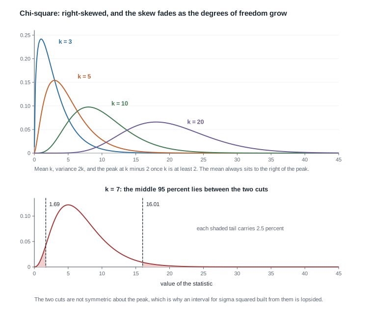
Every member of the family lives on the positive half-line and is right-skewed, because a sum of squares cannot go negative but can grow without bound. As \(k\) grows the peak moves right, the spread grows like \(\sqrt{2k}\), and the skew fades; the mean sits at \(k\) while the mode sits at \(k - 2\) once \(k \ge 2\), so the mean is always to the right of the peak. Hold on to that asymmetry — it is why the variance interval in the second worked example comes out lopsided, and it does not fade at the sample sizes a laboratory actually collects.
The third result is the one worth the derivation.
\[\bar{X} \quad \text{and} \quad S^2 \quad \text{are independent.}\]
This should look surprising. \(S^2\) is built from the same numbers as \(\bar{X}\), and is defined by subtracting \(\bar{X}\) from each of them. Under almost any other model the two are dependent. Under the normal they are not, and that is what lets us divide one by the other in the next subsection and still know the law of the ratio.
Why the mean and the variance come apart
Standardize first, so that the parameters disappear. Put \(Z_i = (X_i - \mu)/\sigma\), so that \(Z_1, \dots, Z_n\) are independent standard normal, and collect them into a vector \(Z\). Choose any \(n \times n\) orthogonal matrix \(A\) whose first row is \((1/\sqrt{n}, \dots, 1/\sqrt{n})\). Such a matrix exists, because the all-ones direction is a unit vector once divided by \(\sqrt{n}\) and Gram-Schmidt extends any unit vector to an orthonormal basis; the classical explicit choice is the Helmert matrix. Set \(Y = AZ\).
Two facts about \(Y\) do the work. First, \(Y\) is again a vector of independent standard normal variables: a linear map of a Gaussian vector is Gaussian, and \(\operatorname{Var}(AZ) = A I_n A^{\top} = I_n\). That is the first place normality enters, and it is essential — for a non-Gaussian \(Z\) the coordinates of \(Y\) would still be uncorrelated, since the covariance calculation is unchanged, but uncorrelated is not independent. Second, an orthogonal map preserves length, so \(\sum_{i=1}^n Y_i^2 = \sum_{i=1}^n Z_i^2\).
Read off the pieces. The first coordinate is
\[Y_1 = \frac{1}{\sqrt{n}} \sum_{i=1}^n Z_i = \sqrt{n}\, \bar{Z},\]
and the remaining coordinates absorb everything else:
\[\sum_{i=2}^n Y_i^2 = \sum_{i=1}^n Z_i^2 - Y_1^2 = \sum_{i=1}^n Z_i^2 - n \bar{Z}^2 = \sum_{i=1}^n (Z_i - \bar{Z})^2 = \frac{(n-1)S^2}{\sigma^2}.\]
Confirm the last two equalities with a pencil: expanding \(\sum (Z_i - \bar{Z})^2\) gives \(\sum Z_i^2 - 2\bar{Z}\sum Z_i + n\bar{Z}^2 = \sum Z_i^2 - n\bar{Z}^2\), and \(Z_i - \bar{Z} = (X_i - \bar{X})/\sigma\) because the shift by \(\mu\) cancels.
Everything now follows. \(Y_1\) is standard normal, so \(\bar{X} = \mu + \sigma Y_1/\sqrt{n}\) is \(N(\mu, \sigma^2/n)\). The sum \(\sum_{i=2}^n Y_i^2\) is a sum of \(n-1\) squared independent standard normal variables, so \((n-1)S^2/\sigma^2\) is \(\chi^2_{n-1}\). And \(Y_1\) is independent of \((Y_2, \dots, Y_n)\), so \(\bar{X}\) and \(S^2\) are independent as functions of separate blocks. That is the second place normality enters, and it is where a general parent would leave you with uncorrelated blocks and no independence.
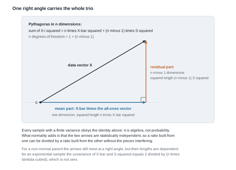
The picture is worth more than the matrix. Think of the sample as one vector in \(n\)-dimensional space. It splits into a piece along the all-ones direction, fixed by \(\bar{X}\) alone, and a residual piece orthogonal to it whose squared length is exactly \((n-1)S^2\). Pythagoras gives \(\sum_i X_i^2 = n\bar{X}^2 + (n-1)S^2\), and the degrees of freedom add the same way, \(n = 1 + (n-1)\). That is algebra, true of any sample. What normality contributes is that the two legs are independent and not merely orthogonal.
The converse holds too: if the parent has finite, non-zero variance and \(\bar{X}\) and \(S^2\) are independent for some \(n \ge 2\), the parent must be normal — a characterization due to Geary and sharpened by Lukacs. Independence here is a defining property, not a convenience. To see how ordinary dependence is, use \(\operatorname{Cov}(\bar{X}, S^2) = \mu_3/n\), where \(\mu_3 = \mathbb{E}[(X - \mu)^3]\) is the third central moment. At \(n = 2\) with \(\mu = 0\) you can check it in three lines: \(S^2 = (X_1 - X_2)^2/2\), so \(\bar{X}S^2\) expands to \(\frac{1}{4}(X_1^3 + X_2^3 - X_1^2 X_2 - X_1 X_2^2)\), whose expectation is \(\mu_3/2\) because each cross term carries a factor \(\mathbb{E}[X_i] = 0\). An exponential parent with rate \(\lambda\) has \(\mu_3 = 2/\lambda^3\), so the covariance is \(2/(n\lambda^3)\) and never vanishes. Exponential data break the independence claim and the chi-square claim together.
Building \(t\) and \(F\) from the pieces
Now put the trio to work. Define
\[Z = \frac{\bar{X} - \mu}{\sigma/\sqrt{n}}, \qquad V = \frac{(n-1)S^2}{\sigma^2}.\]
By the three results, \(Z \sim N(0,1)\), \(V \sim \chi^2_{n-1}\), and \(Z\) and \(V\) are independent. That is precisely the recipe in the definition of the \(t\) distribution, so \(Z/\sqrt{V/(n-1)}\) has the \(t\) distribution with \(n-1\) degrees of freedom. Simplify the left-hand side, using \(V/(n-1) = S^2/\sigma^2\) and \(S \ge 0\):
\[\frac{Z}{\sqrt{V/(n-1)}} = \frac{(\bar{X} - \mu)\sqrt{n}/\sigma}{\sqrt{S^2/\sigma^2}} = \frac{(\bar{X} - \mu)\sqrt{n}/\sigma}{S/\sigma} = \frac{\bar{X} - \mu}{S/\sqrt{n}}.\]
Every \(\sigma\) has cancelled. The quantity on the right can be computed from the data once you supply a candidate value of \(\mu\), and its distribution, \(t_{n-1}\), involves no unknown at all. That is the engine of the first worked example.
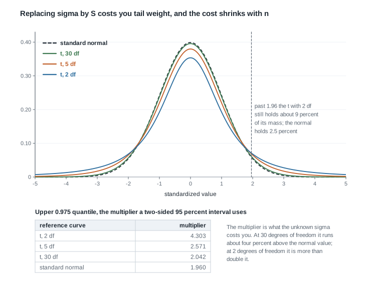
The figure prices the substitution of \(S\) for \(\sigma\). Every \(t\) density is lower at the centre and heavier in the tails than the standard normal, because the random denominator sometimes comes out small and inflates the ratio. Past 1.96 the \(t\) with two degrees of freedom still carries about nine percent of its mass, against the normal’s 2.5 percent. The tabulated multipliers say the same thing in the form you will use: 4.303 at two degrees of freedom, 2.571 at five, 2.042 at thirty, against 1.960 for the normal. By thirty the penalty is about four percent, which is why the normal multiplier passes unnoticed in large samples and burns people in small ones.
The \(F\) distribution comes from the same parts. If \(V_1 \sim \chi^2_{k_1}\) and \(V_2 \sim \chi^2_{k_2}\) are independent, then \((V_1/k_1)/(V_2/k_2)\) has the \(F\) distribution with \(k_1\) and \(k_2\) degrees of freedom. For two independent normal samples of sizes \(m\) and \(n\) the two chi-square variables are the scaled sample variances, and the ratio
\[\frac{S_1^2/\sigma_1^2}{S_2^2/\sigma_2^2} \sim F_{m-1,\; n-1}\]
is again free of every unknown parameter. Squaring a \(t_k\) variable gives an \(F_{1, k}\) variable, which is a good consistency check to run on the two definitions.
Pivots, inversion, and the meaning of coverage
What makes a quantity a pivot
A pivotal quantity is a function \(Q(X, \theta)\) of the data and the parameter whose distribution under \(P_\theta\) is the same for every \(\theta \in \Theta\). It is not a statistic: a statistic can be computed from the data alone but its law generally moves with \(\theta\), while a pivot has a fixed law and cannot be computed, since evaluating it would require knowing \(\theta\).
In the normal model, \((\bar{X} - \mu)/(S/\sqrt{n})\) is a pivot, distributed \(t_{n-1}\) whatever \(\mu\) and \(\sigma\) are, and that is the whole content of the previous section; \((n-1)S^2/\sigma^2\) is a pivot for \(\sigma^2\), distributed \(\chi^2_{n-1}\). By contrast \(\bar{X}\) on its own is a statistic and not a pivot, because its law shifts with \(\mu\) — which is exactly why it estimates \(\mu\) and exactly why it cannot by itself deliver an interval.
Turning a pivot into an interval
Suppose \(Q(X, \theta)\) is a pivot with a known distribution. Pick constants \(a\) and \(b\) with
\[P_\theta\big(a \le Q(X, \theta) \le b\big) = 1 - \alpha \quad \text{for every } \theta,\]
which is possible precisely because the law of \(Q\) does not move with \(\theta\). Now define the random set
\[C(X) = \{\theta \in \Theta : a \le Q(X, \theta) \le b\}.\]
For a fixed \(\theta\), the statement \(\theta \in C(X)\) and the statement \(a \le Q(X, \theta) \le b\) are the same event — the same set of sample outcomes, written twice. Therefore
\[P_\theta\big(\theta \in C(X)\big) = 1 - \alpha \quad \text{for every } \theta,\]
and \(C(X)\) is a confidence set with exact coverage \(1 - \alpha\). Notice how little happened: no approximation, no limit, no new probability, only bookkeeping applied to a distributional fact. Notice also what the probability is over. The randomness sits in \(X\), and \(\theta\) is a fixed unknown constant throughout. That observation is the entire content of the misreading section below.
One caveat. The pair \((a, b)\) is not pinned down by the requirement; any pair with the right probability inverts to a valid interval, and the equal-tailed choice is a convention rather than a derivation. For a symmetric pivot such as the \(t\) it also happens to be the shortest. For a skewed pivot such as the chi-square it is not, and you should know you have chosen convenience over length.
Pivots that have nothing to do with the normal
The construction is not a normal-theory trick. Let \(X_1, \dots, X_n\) be independent Uniform\((0, \theta)\) draws and let \(M = X_{(n)}\) be the sample maximum, whose distribution function you derived in Week 3: \(P_\theta(M \le t) = (t/\theta)^n\) for \(0 \le t \le \theta\). Then for \(0 \le u \le 1\),
\[P_\theta\!\left(\frac{M}{\theta} \le u\right) = u^n,\]
free of \(\theta\), so \(M/\theta\) is a pivot. Inverting with \(a = (\alpha/2)^{1/n}\) and \(b = (1 - \alpha/2)^{1/n}\) turns \(a \le M/\theta \le b\) into \(M/b \le \theta \le M/a\). With \(n = 10\), \(\alpha = 0.05\) and an observed maximum of \(4.7\), the constants are \(a = 0.6915\) and \(b = 0.9975\), and the interval runs from \(4.712\) to \(6.797\). It lies entirely above the observed maximum, as it must, since \(\theta \ge M\) with probability one, and it is wildly asymmetric, because the pivot is. None of this required a derivative, a regularity condition, or a limit — a contrast Week 12 turns into a theorem when the information bound fails to apply to this model at all.
Worked example — a \(t\) interval for a calibration mean
Setting. A calibration laboratory weighs the same reference mass eight times on one balance, recording, in grams,
\[10.2, \quad 9.8, \quad 10.5, \quad 10.1, \quad 9.6, \quad 10.4, \quad 9.9, \quad 10.3.\]
Model the readings as independent \(N(\mu, \sigma^2)\) with both parameters unknown. The estimand is \(\mu\), the balance’s long-run mean reading for this mass. Take \(\alpha = 0.05\).
Step one, the centre. The eight values sum to \(80.8\), so \(\bar{x} = 80.8/8 = 10.1\) grams.
Step two, the spread. Work with the deviations, which must sum to zero — a free arithmetic check you should always run.
| \(x_i\) | \(x_i - \bar{x}\) | \((x_i - \bar{x})^2\) |
|---|---|---|
| 10.2 | \(0.1\) | 0.01 |
| 9.8 | \(-0.3\) | 0.09 |
| 10.5 | \(0.4\) | 0.16 |
| 10.1 | \(0.0\) | 0.00 |
| 9.6 | \(-0.5\) | 0.25 |
| 10.4 | \(0.3\) | 0.09 |
| 9.9 | \(-0.2\) | 0.04 |
| 10.3 | \(0.2\) | 0.04 |
| sum | \(0.0\) | 0.68 |
So \(\sum (x_i - \bar{x})^2 = 0.68\), giving \(s^2 = 0.68/7 = 0.09714\) and \(s = 0.3117\) grams. The estimated standard error of the mean is \(s/\sqrt{8} = 0.3117/2.8284 = 0.11019\) grams.
Step three, the pivot. From the previous section, \(T = (\bar{X} - \mu)/(S/\sqrt{n}) \sim t_7\), whatever \(\mu\) and \(\sigma\) happen to be.
Step four, the cuts. The upper \(0.975\) quantile of \(t_7\) is \(2.3646\), and by symmetry \(P(-2.3646 \le T \le 2.3646) = 0.95\).
Step five, the inversion. Rearranging \(-2.3646 \le (\bar{X}-\mu)/(S/\sqrt{n}) \le 2.3646\) moves \(\mu\) to the middle and gives
\[\bar{X} - 2.3646 \frac{S}{\sqrt{n}} \;\le\; \mu \;\le\; \bar{X} + 2.3646 \frac{S}{\sqrt{n}}.\]
The half-width is \(2.3646 \times 0.11019 = 0.2606\) grams, so the realized interval runs from \(10.1 - 0.2606 = 9.839\) to \(10.1 + 0.2606 = 10.361\) grams.
What it means, and what it assumed. The procedure that produced \((9.839, 10.361)\) captures the balance’s long-run mean reading in 95 percent of repetitions of the whole experiment. It is wider than \(\bar{x} \pm 2 s/\sqrt{n}\) would have been, and the excess is the price of not knowing \(\sigma\) at \(n = 8\). Three assumptions carried it: independence across the eight weighings, a common variance, and normality — and independence is the one a laboratory most often breaks, through drift within a session. Note the estimand, in the Week 1 spirit: this interval is about the balance’s mean reading, not the true mass of the reference. A systematic calibration offset would shift \(\mu\) and the interval together, and no amount of replicate weighing would reveal it.
The same reasoning, transferred
Now two independent normal samples with a shared variance: \(X_1, \dots, X_m\) from \(N(\mu_1, \sigma^2)\) and \(W_1, \dots, W_n\) from \(N(\mu_2, \sigma^2)\), with sample variances \(S_1^2\) and \(S_2^2\) and the estimand \(\delta = \mu_1 - \mu_2\). Everything structural repeats. The difference of means is normal, \(\bar{X} - \bar{W} \sim N(\delta, \sigma^2(1/m + 1/n))\). The two residual sums of squares are independent chi-squares, so their sum is \(\chi^2_{m+n-2}\), and the pooled estimator \(S_p^2 = \{(m-1)S_1^2 + (n-1)S_2^2\}/(m+n-2)\) satisfies \((m+n-2)S_p^2/\sigma^2 \sim \chi^2_{m+n-2}\). The numerator is independent of the denominator, within each sample and across them, so
\[\frac{(\bar{X} - \bar{W}) - \delta}{S_p \sqrt{1/m + 1/n}} \sim t_{m+n-2}\]
is a pivot, and inversion proceeds exactly as before. Suppose \(m = n = 6\) with \(\bar{x} = 12.4\), \(s_1^2 = 0.90\), \(\bar{w} = 11.5\) and \(s_2^2 = 1.30\). Then \(s_p^2 = (5 \times 0.90 + 5 \times 1.30)/10 = 1.10\), so \(s_p = 1.0488\) and the standard error is \(1.0488\sqrt{1/3} = 0.6055\). With \(t_{10}\) giving a multiplier of \(2.2281\), the half-width is \(1.3492\) and the interval for \(\delta\) runs from \(-0.449\) to \(2.249\).
What stayed the same: a standardized quantity in which the unknown scale cancels, a chi-square denominator independent of the numerator, and a purely algebraic inversion. What changed: the degrees of freedom became \(m + n - 2\) because two means were estimated, and a new assumption appeared, that the two populations share \(\sigma^2\). The reading changed too. The interval contains zero, so these data do not separate the two means — a statement about resolution at this sample size, not evidence that the means are equal.
Second worked example — a chi-square interval for a normal variance
Setting. Keep the eight calibration weighings and change the estimand. A metrologist wants the balance’s repeatability, \(\sigma\), reported as a 95 percent interval for \(\sigma^2\). The sample gave \(\sum (x_i - \bar{x})^2 = 0.68\) and \(s^2 = 0.09714\).
Step one, the pivot. From the trio, \(V = (n-1)S^2/\sigma^2 \sim \chi^2_7\), with observed numerator \((n-1)s^2 = 0.68\). This pivot is not symmetric and no standardization makes it so.
Step two, the cuts. The equal-tailed choice takes the \(0.025\) and \(0.975\) quantiles of \(\chi^2_7\), which are \(1.6899\) and \(16.0128\) — the two cuts drawn in the lower panel of the chi-square figure above.
Step three, the inversion. Start from \(1.6899 \le 0.68/\sigma^2 \le 16.0128\). All three quantities are positive, so taking reciprocals reverses the inequalities and multiplying through by \(0.68\) gives
\[\frac{0.68}{16.0128} \;\le\; \sigma^2 \;\le\; \frac{0.68}{1.6899},\]
that is, \(0.0425 \le \sigma^2 \le 0.4024\) in grams squared. Taking square roots, which is legitimate because the map is increasing on the positive half-line, the interval for \(\sigma\) itself runs from \(0.206\) to \(0.634\) grams.
Reading the asymmetry. The estimate \(s^2 = 0.0971\) sits far from the middle: the interval extends \(0.0547\) below it and \(0.3053\) above it, a factor of about \(5.6\). Nothing has gone wrong. The chi-square pivot is right-skewed, and inverting a skewed pivot through a reciprocal produces a long upper arm. Substantively, eight weighings pin down a lower bound on repeatability reasonably well and an upper bound hardly at all. Reporting \(s^2\) plus or minus something symmetric would have hidden that.
Two critiques. First, the equal-tailed cuts are a convention; other pairs with the same enclosed probability exist, some giving shorter intervals. Second, and more serious, this interval is far less robust than the \(t\) interval. The \(t\) pivot leans on normality mainly through \(\bar{X}\), which the central limit theorem partially rescues; the chi-square pivot leans on fourth-moment behaviour, which nothing rescues. Applying both recipes to exponential data at \(n = 8\) gives roughly 89 percent coverage for the \(t\) interval and under 80 percent for this one — worth remembering every time someone reports an interval for a variance component.
A simulation check you can run
Derive, then compute, then critique. The claim “this recipe covers \(\mu\) in 95 percent of repetitions” is directly checkable, and checking it is the fastest way to make coverage stop feeling abstract. In R, the whole experiment is a few lines.
set.seed(20260405)
reps <- 20000; n <- 8; mu <- 10; sigma <- 0.3

correct <- replicate(reps, {
  x    <- rnorm(n, mu, sigma)
  half <- qt(0.975, df = n - 1) * sd(x) / sqrt(n)
  abs(mean(x) - mu) <= half
})
mean(correct)   # close to 0.950

naive <- replicate(reps, {
  x <- rnorm(n, mu, sigma)
  abs(mean(x) - mu) <= 1.96 * sd(x) / sqrt(n)
})
mean(naive)     # close to 0.909
The first proportion lands near \(0.950\) and the second near \(0.909\). The second is not simulation noise: \(P(|T_7| \le 1.96) = 0.9092\) exactly, so the normal multiplier costs four percentage points of coverage at this sample size. Replace rnorm(n, mu, sigma) with rexp(n, rate = 1) and compare against that draw’s true mean of 1; the first proportion drops to about \(0.894\), which is the misspecification effect from the previous section rather than an error in the code.
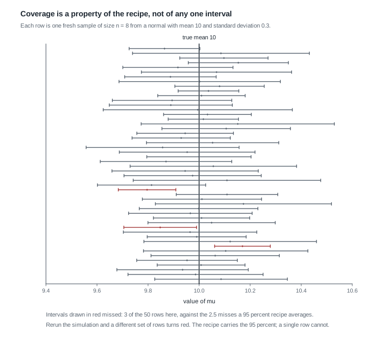
The figure draws fifty of those repetitions instead of counting twenty thousand. Each row is a fresh sample of eight observations and the interval it produced; the vertical line is the true mean, fixed at 10 and never moving. Three rows missed here, against an average of two and a half. Two things reward a stare. The widths differ visibly, because each interval uses its own \(s\), and the widest are not the ones that miss; the misses are samples whose \(s\) came out small enough to produce a short interval in the wrong place. Coverage is a property of the column, not of any row.
The misreading to avoid
Here is the sentence, more or less verbatim, that a graduate student writes every year:
“We are 95 percent confident that \(\mu\) is between 9.839 and 10.361, so there is a 95 percent probability that the true mean lies in that range.”
The first clause is fine: “confident” is a term of art meaning the procedure has 95 percent coverage. The second clause is a different claim, and in this framework it is not available. The probability statement \(P_\mu(\mu \in C(X)) = 0.95\) is an integral over \(X\) with \(\mu\) held fixed. Once the eight weighings are in hand, \(C(x)\) is the fixed pair \((9.839, 10.361)\) and \(\mu\) is a fixed unknown constant, so \(9.839 \le \mu \le 10.361\) is either true or false with no random element left to carry a probability. Writing \(0.95\) beside it silently changes what kind of object \(\mu\) is.
If that feels like pedantry, this example should dislodge it. Let \(X_1, X_2\) be independent draws from Uniform\((\theta - 1/2,\, \theta + 1/2)\) and report \((\min(X_1, X_2),\, \max(X_1, X_2))\). Its coverage is exactly one half, since \(\theta\) lies between the two observations precisely when one falls below it and the other above, and each falls below with probability one half independently. So this is a bona fide 50 percent procedure. Now suppose the observations differ by at least \(1/2\), say \(x_1 = 0.1\) and \(x_2 = 0.7\). Each lies within \(1/2\) of \(\theta\), so \(\theta \gt x_2 - 1/2 = 0.2 \ge x_1\) and \(\theta \lt x_1 + 1/2 = 0.6 \le x_2\): the reported interval contains \(\theta\) with certainty. A gap that wide happens a quarter of the time; on the other three quarters, where the gap falls below \(1/2\), the conditional coverage is only one third. The 50 percent is an average over two very different situations, and attaching it to the interval in front of you is the wrong arithmetic.
A quieter misreading is worth naming too: the interval is not a range for the observations. It is an interval for \(\mu\) and shrinks like \(n^{-1/2}\), whereas a range built to contain a future measurement does not shrink to a point.
None of this makes the probability sentence wrong in every framework — it makes it wrong here. Give \(\mu\) a prior and the posterior is a genuine distribution for \(\mu\) given the data, so “the probability that \(\mu\) lies in this interval is 0.95” becomes a legitimate within-model statement about a credible interval. That object arrives in Week 9, and Week 13 sets the two side by side on the same data. Until then, keep the two sentences apart.
Practice on your own
A density by transformation. From the \(\chi^2_{n-1}\) density, use a change of variables to write down the density of \(S^2\) for a normal sample. Confirm that \(\mathbb{E}[S^2] = \sigma^2\) and \(\operatorname{Var}(S^2) = 2\sigma^4/(n-1)\), and say why the second shrinks like \(1/n\) while the first does not shrink at all.
An audit. A colleague writes: “Since \((n-1)S^2/\sigma^2 \sim \chi^2_{n-1}\) and a chi-square with \(n-1\) degrees of freedom has variance \(2(n-1)\), we get \(\operatorname{Var}(S^2) = 2\sigma^4/(n-1)\); taking square roots, \(\operatorname{Var}(S) = \sigma^2\sqrt{2/(n-1)}\).” One conclusion is right and one is badly wrong. Identify which, explain the step that fails, and describe a simulation that would settle it.
A counterexample hunt. Find a non-normal parent for which \(\bar{X}\) and \(S^2\) are uncorrelated but not independent. Use \(\operatorname{Cov}(\bar{X}, S^2) = \mu_3/n\) to see which parents kill the covariance, then take a bounded symmetric parent such as Uniform\((-1, 1)\) and argue dependence directly: what does \(|\bar{x}|\) close to one force \(s^2\) to be?
A simulation to describe. Predict, before running anything, whether the equal-tailed chi-square interval for \(\sigma^2\) over-covers or under-covers when the parent has heavier tails than the normal, say a \(t\) with five degrees of freedom scaled to variance one. Write out the simulation, name the quantity you would report, and say what would falsify your prediction.
Another inversion. Invert the pivot \((S_1^2/\sigma_1^2) / (S_2^2/\sigma_2^2) \sim F_{m-1, n-1}\) into a \(1 - \alpha\) interval for the variance ratio \(\sigma_1^2/\sigma_2^2\). State which quantiles you need, and check the interval behaves sensibly when the two sample variances happen to be equal.
Where to read more
- MIT OpenCourseWare 18.650, Statistics for Applications for normal theory, the \(t\) multiplier, and intervals treated as a construction rather than a formula.
- MIT OpenCourseWare 18.655, Mathematical Statistics for the general pivot idea and the decision-theoretic setting Weeks 9 and 11 will need.
- Penn State STAT 414 for a slower treatment of the chi-square, \(t\) and \(F\) densities, including the derivations this page quotes without proving.
- The R Project for
qt,qchisqandqf, the source of every multiplier above. - Hogg, McKean and Craig cover the sampling distributions in their third chapter and interval estimation in their fourth.
- Course pages: the syllabus, the schedule, and the resources page.
Where this goes next
Everything here is exact, and everything here is fragile in the same way: it assumed a normal model. Week 5 removes that assumption. What comes through is built from convergence in probability and in distribution, the weak law, the central limit theorem and the delta method, and its practical shape is that \((\bar{X} - \mu)/(S/\sqrt{n})\) is approximately standard normal for large \(n\) under conditions far weaker than normality. The word approximately does real work there, and Week 5 spends its time on how much. Read this week’s exact results as the standard those approximations are measured against, and Week 3 as the source of the order-statistic facts behind the uniform pivot.
Two threads run forward. The coverage discussion is a promissory note that Week 9 redeems with the posterior, the one object for which the forbidden sentence is true. And the uniform pivot, needing no derivatives and no regularity, is a first hint of Week 12, where that same model falls outside the Cramer-Rao conditions entirely. The notes index lists every unit in order.