Week 15 — Project workshop & synthesis

Closing the loop: the whole arc in one checklist, and how to finish your report well

The week question

When your final Bayesian analysis is finished, how do you know it is finished — and could a stranger re-run it and trust the conclusion?

That is the workshop question for the last week of the term. There is no new theory here. Everything you need has already appeared: this week is about assembling it, recognizing a complete analysis when you see one, and getting your report and your studying for the cumulative final into good shape.

Where we are and why this matters

This is the final week, so we look back across the entire arc rather than forward to new machinery. The term moved through one long story, and naming its chapters is the first study act:

Plausibility (Weeks 1–2). Reasoning under uncertainty, and discrete Bayes’ rule through diagnostic testing — belief as something you update, not something you fix.
The working trio (Weeks 3–5). Prior \(f(\theta)\), likelihood \(L(\theta \mid y)\), and posterior \(f(\theta \mid y)\) as a system; the Beta-Binomial model for a proportion; prior sensitivity and posterior summaries.
Prediction and computation (Weeks 6–7). The posterior predictive for a future observation, and simulation-first computation that reproduces closed forms when they exist and substitutes for them when they do not.
Regression (Weeks 9–11). The unknown grew from one proportion into a relationship: priors on the coefficients of \(y_i = \beta_0 + \beta_1 x_i + \varepsilon_i\), with each coefficient reported as a posterior mean and a credible interval, plus model checking.
Hierarchy and decisions (Weeks 12–14). Partial pooling across groups — group estimates shrinking toward an overall mean, more so for small or noisy groups — and turning a posterior into a decision you can defend and communicate.

The recurring bike-to-campus survey threaded through all of it, so you have watched one problem grow from a tally table into a full model with predictions, checks, and a plain-language conclusion. That growth is the course. The final report asks you to do the same thing once, start to finish, on a question of your own; the cumulative final asks you to do the moves on demand. Consolidating now is what makes both feel like recall rather than discovery.

Learning goals

By the end of this workshop week you should be able to:

Restate the course arc as one pipeline — plausibility → model → posterior → prediction/checking → regression → hierarchy → decision/communication — and say what each stage contributes.
Apply a definition-of-done checklist to your own analysis and spot what is missing.
Run a compact end-to-end analysis (the bike case) from prior to posterior to a posterior-predictive check, getting the Beta-Binomial arithmetic right.
Recognize the same complete pipeline in a different model (a regression recap), proving the checklist is model-independent.
Name the end-of-term mistakes that most often weaken an otherwise good report, and how to catch each.
Read a Bayesian conclusion as a statement under a model, and write one that an honest non-technical reader could trust.

Core vocabulary

A recall list — nothing new, the working set of the whole term gathered for one last pass. If any term is fuzzy, that is your study signal.

Prior \(f(\theta)\) — belief about the unknown \(\theta\) before the data.
Likelihood \(L(\theta \mid y)\) — how compatible each value of \(\theta\) is with the observed data; a function of \(\theta\), not a distribution over \(\theta\).
Posterior \(f(\theta \mid y)\) — updated belief after the data, via \(f(\theta \mid y) \propto L(\theta \mid y)\, f(\theta)\); the goal object.
Credible interval — an interval that, given data and model, contains \(\theta\) with stated posterior probability (contrast: a confidence interval describes the long-run behavior of the procedure).
Posterior predictive — the distribution of a new observation, obtained by averaging the data model over the posterior.
Posterior-predictive check — comparing data simulated from the fitted model against the actual data to judge model adequacy.
Partial pooling / shrinkage — group estimates pulled from their no-pooling values toward the overall mean, more for small or noisy groups.
Reproducible report — a .qmd where code, output, and interpretation live together, with seeded randomness, so the result regenerates on someone else’s machine.

The whole arc as one pipeline

Every problem this term was the same pipeline at a different scale. State it once, and the course collapses into something memorable.

Plausibility → a model. Translate background belief into a prior \(f(\theta)\) and choose a data model (the likelihood). For a proportion that is Beta + Binomial; for counts, Gamma + Poisson; for a relationship, priors on regression coefficients with a Normal noise model.
Combine → a posterior. Apply \(f(\theta \mid y) \propto L(\theta \mid y)\, f(\theta)\). The \(\propto\) drops the evidence \(f(y)\), a constant in \(\theta\) that only rescales — harmless until you need an actual probability, at which point you normalize (or simulate).
Summarize honestly. Report a point estimate (posterior mean or median) with a credible interval. Never a point alone.
Predict and check. Form the posterior predictive for a future observation, then run a posterior-predictive check: does data simulated from the fitted model look like the data you actually saw?
Communicate and decide. Say what the result means and what it does not, name the assumptions, and translate it into a defensible action or a plain-language conclusion.

Regression and hierarchy did not change these five moves — they only changed what \(\theta\) is. In regression \(\theta\) is a set of coefficients; in a hierarchical model \(\theta\) includes both group-level and population-level quantities, and partial pooling falls out of the same posterior logic. That portability is the single most testable idea of the term.

Definition of done: a checklist for a good Bayesian analysis

Use this as the gate on your final report. An analysis is done when every box can be checked honestly:

State the model. The prior \(f(\theta)\) and the likelihood \(L(\theta \mid y)\) are both written down, with a sentence on why each is reasonable. (A reader should be able to disagree with your prior — which means you have to show it.)
Fit it. Produce the posterior \(f(\theta \mid y)\), either in closed form (conjugate cases) or by simulation, with randomness seeded.
Summarize with an interval. Every reported quantity is a point estimate paired with a credible interval — never a lone number.
Check the model. At least one posterior-predictive check, with an honest read: does the model reproduce the salient features of the data, and where does it fall short?
Run a sensitivity glance. Note whether a reasonable change of prior would move the conclusion. If it would not, you may call the result data-driven; if it would, say so.
Conclude in plain language. A short, caveated statement a non-technical reader could act on, with the model named as part of the claim.
Make it reproducible. A single .qmd that renders cleanly: code, output, and prose together; seeds set; session info included.

If a box is unchecked, the analysis is not finished — it is a draft. This checklist is also the most reliable way to study for the final: each box maps to a move you must be able to perform.

Worked example — bike-to-campus, a complete mini-analysis (recurring case)

This is the running survey: we estimate \(\theta\), the proportion of students who bike to campus, and walk every checklist box.

State the model. Background belief is weak, so use the mild prior \(f(\theta) = \text{Beta}(2,2)\), whose mean is \(2/(2+2) = 0.5\) — a gentle pull to the middle, easily overridden. The data are counts of bikers in a fixed survey, so the likelihood is Binomial: \(L(\theta \mid y) \propto \theta^{\,y}(1-\theta)^{\,n-y}\).

Fit it. We surveyed \(n = 24\) students and found \(y = 8\) bikers. Beta-Binomial updating adds successes to the first shape and failures to the second: \[ \theta \mid y \;\sim\; \text{Beta}(\alpha + y,\; \beta + n - y) \;=\; \text{Beta}(2 + 8,\; 2 + 16) \;=\; \text{Beta}(10, 18). \]

Summarize with an interval. The posterior mean is \[ \frac{\alpha + y}{\alpha + \beta + n} \;=\; \frac{10}{10 + 18} \;=\; \frac{10}{28} \;\approx\; 0.357, \] paired with a 90% credible interval from the Beta(10,18) quantiles (computed below, roughly 0.23 to 0.50). Headline: about 36% of students bike, plausibly between ~23% and ~50%.

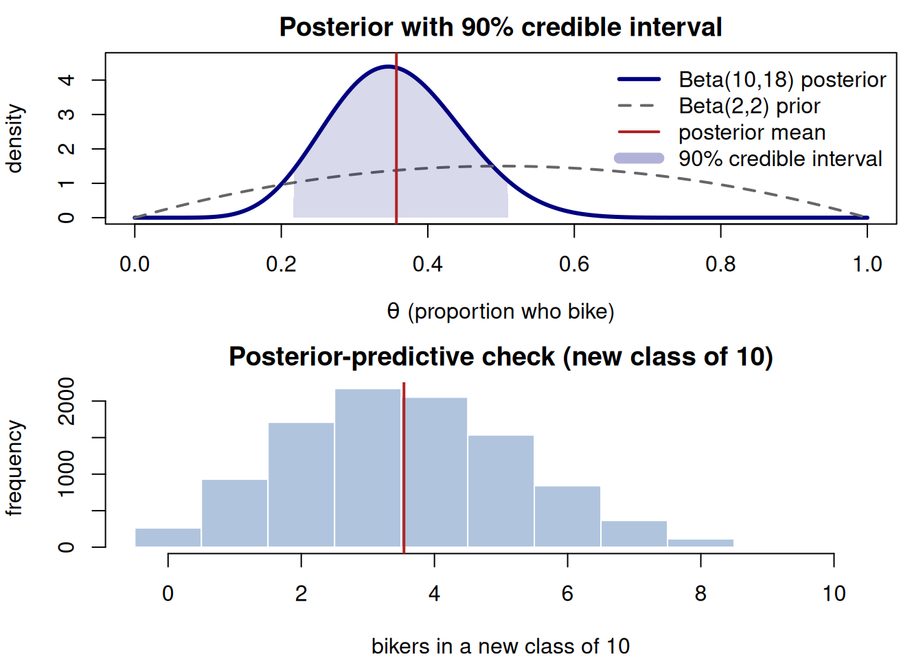
Check the model and predict. A posterior-predictive check for a new class of 10 students: simulate \(\theta\) from the posterior, then a Binomial count from each \(\theta\), and see whether the spread of simulated counts is consistent with what we’d expect (centered near \(10 \times 0.357 \approx 3.6\), but wider than a plain Binomial because it carries our remaining uncertainty about \(\theta\)).

Sensitivity glance. Swapping the mild Beta(2,2) for a flat Beta(1,1) gives Beta(9,17), mean \(9/26 \approx 0.346\) — essentially the same story, so the conclusion is data-driven.

Conclude. Under a mild prior and this 24-student survey, we estimate about 36% of students bike (90% credible interval roughly 23%–50%); a future class of 10 would most plausibly have around 3–4 bikers, with real spread. The figure below draws the posterior, shades the interval, and confirms the predictive by simulation.

set.seed(15)

# --- posterior summaries (closed form) ---
ci        <- qbeta(c(0.05, 0.95), 10, 18)   # 90% credible interval
post_mean <- 10 / 28

theta <- seq(0, 1, length.out = 600)
prior <- dbeta(theta, 2, 2)
post  <- dbeta(theta, 10, 18)

par(mfrow = c(2, 1), mar = c(4, 4, 2, 1))

# top panel: prior, posterior, mean, credible interval
plot(theta, post, type = "l", lwd = 3, col = "navy",
     xlab = expression(theta ~ "(proportion who bike)"),
     ylab = "density", main = "Posterior with 90% credible interval",
     ylim = c(0, max(post) * 1.05))
lines(theta, prior, lwd = 2, lty = 2, col = "gray40")
inside <- theta >= ci[1] & theta <= ci[2]
polygon(c(ci[1], theta[inside], ci[2]),
        c(0, post[inside], 0),
        col = rgb(0, 0, 0.5, 0.15), border = NA)
abline(v = post_mean, lwd = 2, col = "firebrick")
legend("topright", bty = "n",
       legend = c("Beta(10,18) posterior", "Beta(2,2) prior",
                  "posterior mean", "90% credible interval"),
       col = c("navy", "gray40", "firebrick", rgb(0, 0, 0.5, 0.3)),
       lwd = c(3, 2, 2, 8), lty = c(1, 2, 1, 1))

# bottom panel: posterior predictive for a new class of 10
draws    <- rbeta(10000, 10, 18)          # posterior draws of theta
new_bike <- rbinom(10000, size = 10, prob = draws)  # predictive counts
hist(new_bike, breaks = -0.5:10.5, col = "lightsteelblue", border = "white",
     xlab = "bikers in a new class of 10", ylab = "frequency",
     main = "Posterior-predictive check (new class of 10)")
abline(v = mean(new_bike), lwd = 2, col = "firebrick")

# print closed-form vs simulated agreement
cat("closed-form mean:", round(post_mean, 3),
    "| simulated mean:", round(mean(draws), 3), "\n")

closed-form mean: 0.357 | simulated mean: 0.357

cat("closed-form 90% CI:", round(ci, 3),
    "| simulated 90% CI:", round(quantile(draws, c(0.05, 0.95)), 3), "\n")

closed-form 90% CI: 0.217 0.509 | simulated 90% CI: 0.217 0.508

cat("predictive mean bikers /10:", round(mean(new_bike), 2), "\n")

predictive mean bikers /10: 3.54

Two stacked panels. The top panel is a density plot on the proportion axis from 0 to 1: a tall Beta(10,18) posterior curve peaks near 0.35, a dashed low Beta(2,2) prior sits across the middle, a vertical line marks the posterior mean near 0.357, and the region from about 0.23 to 0.50 under the posterior is shaded for the 90 percent credible interval. The bottom panel is a histogram of the number of bikers out of 10 in a new class, centered near 3 to 4 and spread from 0 to about 8. — Figure 1: A complete bike-to-campus mini-analysis: the Beta(10,18) posterior with its mean (~0.357) and shaded 90% credible interval, and the posterior-predictive distribution of bikers in a new class of 10.

The printed lines make “done” concrete: the simulated posterior mean and interval match the closed form, and the predictive panel shows the future-count uncertainty you must report alongside the parameter estimate.

Worked example — study-hours and exam-score, a regression recap (transfer recap)

To prove the checklist is about the moves and not the Beta-Binomial, recap the same definition-of-done on a regression — the secondary recurring case where weekly study-hours (\(x\)) predict exam-score (\(y\)). No new theory, just the checklist in a new model.

State the model. \(y_i = \beta_0 + \beta_1 x_i + \varepsilon_i\) with priors on the intercept \(\beta_0\), the slope \(\beta_1\), and the noise sd — for instance weakly-informative priors centered at “no effect” so the data drive the slope. The likelihood is Normal noise around the line.

Fit it. The posterior is now over the coefficients (and the noise sd) jointly, obtained by simulation with the course packages. Suppose the fit returns a slope posterior with mean about \(4.5\) points per study-hour.

Summarize with an interval. Report the slope as a posterior mean with a credible interval, e.g. each extra weekly study-hour is associated with about 4.5 more exam points (90% credible interval roughly 2.8 to 6.2). A point estimate alone — “4.5 points” — would be incomplete and is exactly the kind of thing a final-report check catches.

Check the model. A posterior-predictive check overlays exam scores simulated from the fitted model on the observed scores; if the simulated spread brackets the real data, the model is adequate for the claim. Note where it is not — say, if real scores fan out more at high study-hours than the constant-variance model allows.

Conclude. Within the range we observed, more study-hours predict higher scores, about 4.5 points each, with honest uncertainty; this is association under a linear model, not a guarantee for any one student. Not one idea changed from the bike case — only what \(\theta\) is. That is the portability the final rewards.

The fit itself uses the course modeling package, so it is shown as illustrative display code, not executed here:

# illustrative — runs with the course packages
fit <- stan_glm(score ~ hours, data = study_data,
                family = gaussian(), seed = 15)
posterior_interval(fit, prob = 0.90)   # slope posterior mean with a credible interval
pp_check(fit)                          # posterior-predictive check vs observed scores

A common mistake

These are the end-of-term traps that most often weaken an otherwise solid report. Review them as a set — a final tends to probe the seam between two.

Calling a draft “done.” An analysis with a posterior but no model check, or a number with no interval, is unfinished. Catch it: run the definition-of-done checklist before you submit; an unchecked box is a to-do, not a stylistic choice.
Reporting a point estimate alone. A posterior mean of 0.357, or a slope of 4.5, with no credible interval hides all the uncertainty. Catch it: never let a single number leave the page without an interval beside it.
Conflating credible and confidence intervals. A 90% credible interval is a direct probability statement about this \(\theta\) given the data; a confidence interval is about the procedure’s long-run coverage. Catch it: if you wrote “90% chance \(\theta\) is in here,” make sure the interval truly came from the posterior.
Confusing the posterior with the posterior predictive. The posterior is about the parameter; the predictive is about a future observation and is wider. Catch it: ask “am I describing \(\theta\) or a future \(y\)?” before stating a number.
Hiding the model, especially the prior. A conclusion stated as a bare fact lets no one judge it. Catch it: name the prior and likelihood in the conclusion sentence — a Bayesian result is a statement under a model.
A report that will not re-run. Unseeded randomness, missing data, or package code that errors makes the work unreproducible. Catch it: render the .qmd from scratch in a clean session before you submit.

Interpretation guidance

When your final report says “about 36% bike, 90% credible interval ~0.23 to 0.50,” here is what that does and does not mean — and the standard your conclusion should meet.

It does mean: given your stated prior, your data, and your model, there is a 90% posterior probability the true proportion lies between roughly 0.23 and 0.50, with the most central single guess near 0.357.
It does not mean: that exactly 36% of this sample biked (the raw rate was \(8/24 \approx 0.333\); the posterior mean is pulled slightly toward the prior). It is not a confidence interval, and it does not say the next class will fall between 23% and 50% — that future-sample question is the predictive, which is wider.
It does carry its assumptions: a strongly informative prior, or a non-representative sample, would move the number. The sensitivity glance is what licenses “data-driven.”

For your report’s plain-language conclusion, the standard is honest and actionable: state the headline with its interval, name the model in the same breath, and flag the one or two assumptions a skeptical reader would most want to push on. A Bayesian conclusion is not a fact about the world; it is a defensible statement under a model, said plainly.

Practice (ungraded)

Check-your-understanding prompts — no answer keys here; work them, then test yourself against the worked examples and the checklist above.

Take a fresh survey of 5 bikers in 12 students. Starting from Beta(2,2), write the posterior and its mean, then name which definition-of-done boxes you would still need to check before calling it finished.
In one sentence, explain what the \(\propto\) in \(f(\theta \mid y) \propto L(\theta \mid y)\,f(\theta)\) drops and why dropping it is harmless.
A draft reports a regression slope of “4.5 points per study-hour” with no interval and no model check. List exactly which checklist boxes are unchecked and what each would add.
Restate this sentence correctly: “The 90% credible interval means there’s a 90% chance the procedure caught the true value.”
Without computing, say which is wider — the posterior for \(\theta\) or the posterior predictive for next class’s biker count — and why, in terms of “what each one is about.”
Sketch in words how you would run a posterior-predictive check for the bike case and what you would conclude if the simulated counts looked nothing like the data.
For your own project topic, write the one-sentence model statement (prior + likelihood) you would put at the top of the report.

Reading guide

This week maps back across the entire spine rather than to one new chapter — use it as a finishing-and-revision plan. From Bayes Rules! (Vitalk, Dogucu & Hu; CC BY-NC-SA 4.0): Chapters 1–2 ground the plausibility-updating mindset and the discrete Bayes’ rule the central identity generalizes; Chapters 3–5 are the conjugate models behind the bike case and its count analogue; Chapters 6–9 cover approximation, posterior summaries, posterior prediction, and model evaluation — the basis for the definition-of-done’s “summarize,” “predict,” and “check” boxes; Chapters 9–13 develop Bayesian regression (the study-hours recap); and the later chapters (roughly 14–17) build hierarchical models and the decision/communication mindset that closes the arc. Re-read each chapter’s summary first; open a section only where your self-check or an unchecked report box flags a gap. Read for the pattern — the five moves recurring across models — not for any single example.

Public vs. graded

These notes and the practice prompts are public and ungraded; no answer keys are posted here. The final report’s specification, rubric, weighting, point values, checkpoint and submission dates, and the cumulative final’s exact format all live in the LMS, and the LMS (Blackboard) is authoritative for every graded specific. The public project-spec shape is a skeleton only; where this page and the LMS differ, the LMS wins.

Looking ahead

This is the last instructional week, so there is no next week to bridge to — only the finish line. The cumulative final exam asks you to run the five moves on demand across the whole arc: set up a conjugate model, update and summarize with a credible interval, reason about a posterior predictive, read a regression coefficient, and diagnose a stated misconception. The definition-of-done checklist and the two recaps above are your most efficient review; rehearse the bike case end to end without notes, then prove to yourself you can transplant the same moves onto a regression. Finish your report against the checklist, then study the moves until they are recall.