Fit a line to synthetic study-hours/exam-score data and read coefficients with their uncertainty
Purpose. This lab is the hands-on companion to Week 09 — Bayesian regression I. There you wrote the model \(y_i = \beta_0 + \beta_1 x_i + \varepsilon_i\) and saw that the posterior is a distribution over the coefficients. Here you produce a fitted line from synthetic data, read the slope and intercept, and — using simulation — turn the single line into a sense of the uncertainty around it.
Goal
Fit a simple regression to synthetic study-hours/exam-score data, and read coefficient estimates with their uncertainty. By the end you will have (1) a scatterplot with a fitted line, (2) numeric estimates of intercept and slope, and (3) an interval around the slope, all reproduced from a seeded, re-runnable .qmd.
Setup
First, make sure your local toolchain is ready: R, VS Code, and Quarto, following the R + VS Code + Quarto setup page. Then, create a new file named lab-09.qmd, paste the chunks below in order, and render. Every chunk uses base R only — no add-on packages — so it runs on a clean install. Seeds are fixed so your numbers match the text.
Steps
Step 1 — Simulate the data
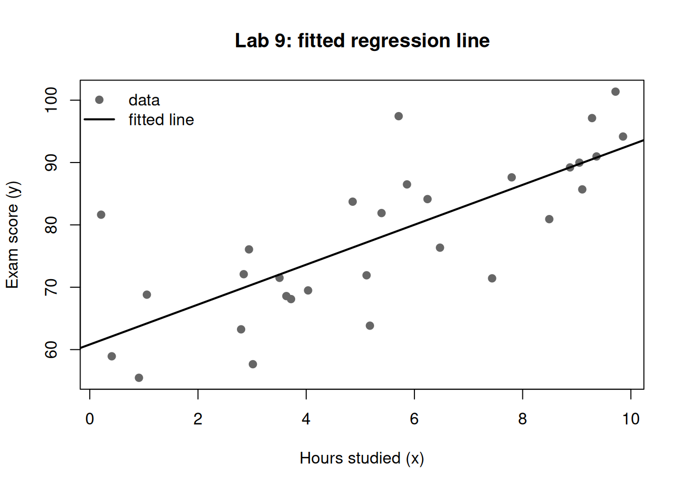
We invent a known truth — intercept \(55\), slope \(4\), noise sd \(8\) — then draw 30 students. Keeping the truth known lets you later check that your estimates recover it.
Fit the least-squares line with lm(). As Week 9 explained, this single line is the likelihood-dominated center of the Bayesian posterior when priors are weak.
Figure 1: Synthetic study-hours vs. exam-score data with the least-squares fit overlaid.
Step 3 — Read the coefficients and a classical interval
lm() gives a point estimate per coefficient and a standard error. We can build a quick interval for the slope to anchor intuition. (A full Bayesian credible interval comes from the posterior in Step 4; here we just read what the data alone say.)
round(coef(fit), 3) # intercept (b0) and slope (b1)
(Intercept)           x
     60.821       3.200
round(confint(fit, "x", level =0.95), 3) # classical 95% interval for the slope
  2.5 % 97.5 %
x 2.152  4.249
Step 4 — Approximate the slope’s uncertainty by simulation
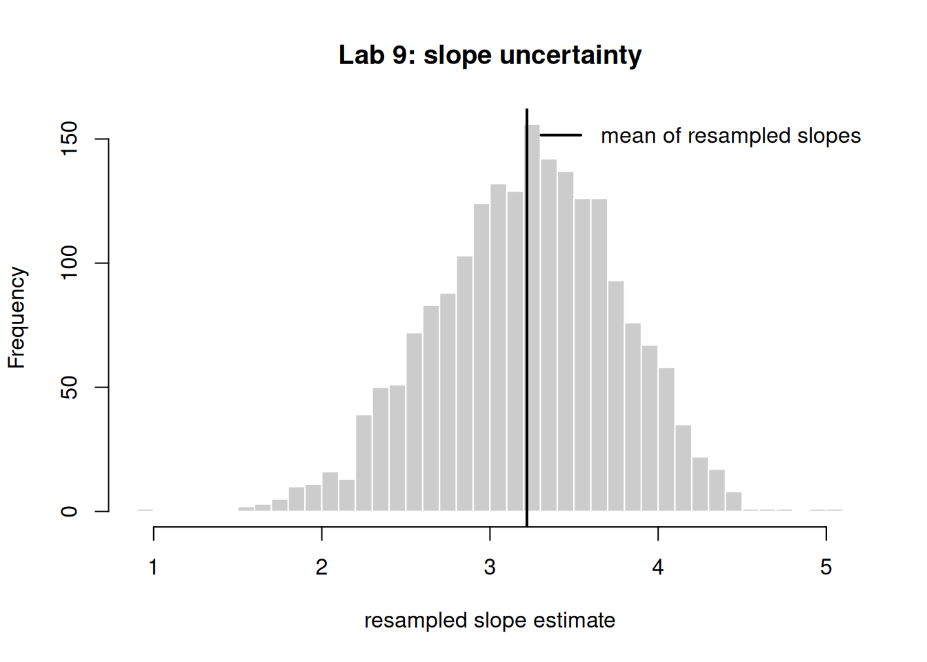
To see “a distribution over lines” without add-on packages, we use a simple resampling loop: repeatedly resample the rows (with replacement), refit, and collect the slope. The spread of these slopes mimics the posterior spread when the prior is weak — the simulation idea you met in Week 7, now applied to a coefficient.
Figure 2: Distribution of the fitted slope across 2000 resamples of the data; the spread visualizes coefficient uncertainty.
Report the slope the way Week 9 insists: a center with an interval, e.g. “about 4 points per hour, with a 95% interval of roughly \([\,\text{lower},\ \text{upper}\,]\).”
Illustrative — the same fit with the course packages
The block below is illustrative only — it runs with the course packages (rstanarm, bayesrules) and is not executed here. It shows the genuine Bayesian fit you would run once those packages are installed; it returns a posterior over the coefficients directly.
# illustrative — runs with the course packages, not executed in this lablibrary(rstanarm)model <-stan_glm( y ~ x,data =data.frame(x = x, y = y),family = gaussian,prior_intercept =normal(55, 10),prior =normal(4, 2),prior_aux =exponential(1/8),seed =909)posterior_interval(model, prob =0.95) # credible intervals for b0 and b1
Verify
Your work is on track if all three hold:
The fitted intercept and slope from Step 2 are near the true values 55 and 4 (within a point or two), confirming the data recover the truth.
In Step 4, the mean of the resampled slopes sits close to the lm() slope from Step 2 — the simulation center matches the closed-form least-squares estimate. (Concrete success criterion: abs(mean(slopes) - coef(fit)[2]) < 0.3.)
The 2.5%–97.5% resample interval for the slope excludes 0, matching the conclusion that study hours have a credible positive effect.
If any check fails, see the next section.
When it breaks
could not find function "lm" or a blank plot — you likely ran the chunk before R finished loading; fix by rendering the whole .qmd top to bottom so chunks execute in order.
Numbers don’t match the text — confirm the set.seed(909) line ran in the same chunk before the random draw; a missing or moved seed is the most common error here. Troubleshoot by re-rendering from a clean session.
object 'fit' not found in Step 4 — Step 2 did not run; chunks share state only when executed in sequence. Render the full document, not a single chunk.
If confint() fails, your lm object is missing; re-run Step 2 first.
AI use note
Tool
Purpose
Verification
LLM assistant (e.g. Claude)
Explain an R error message or suggest a base-R plotting tweak
Re-render the chunk yourself; confirm the figure and printed numbers match the Verify criteria before trusting any AI-suggested edit.
Disclose AI assistance per the syllabus. AI may help you understand code; the runnable result and its interpretation must be your own and must pass the Verify checks.
The graded deliverable, its rubric, point values, and due date live in the LMS (Blackboard), which is authoritative. None of those are posted here; this lab is the public, ungraded practice path.