Build, sample, and verify a posterior on a grid, then render it as a reproducible report
Purpose. This lab puts Week 07 into your hands: you will approximate the bike-proportion posterior on a grid, draw from it, check the simulated mean against the closed-form Beta posterior, and assemble the whole thing as a seeded, reproducible Quarto report. Because this problem is conjugate, you can verify every approximation against a known truth — which is the habit the lab is really teaching.
Goal
Approximate a posterior on a grid, draw from it, compare to the exact Beta, and assemble a reproducible Quarto report. Concretely, by the end you will have a single .qmd that:
builds a grid approximation of the bike-proportion posterior,
samples posterior draws and summarizes them (mean and 95% credible interval),
overlays the grid result on the exact \(\text{Beta}(10,18)\) posterior, and
renders cleanly to HTML with a session record.
Setup
Confirm your local toolchain runs before you start: R must be discoverable by Quarto. If a render complains it cannot find R, work through the setup page first (put R’s bin on PATH, set QUARTO_R, or render from a shell that already has R on PATH). Everything below is base R only — no add-on packages — so once R renders a trivial chunk, you are ready.
Create a new file lab07.qmd and copy the steps into it as chunks. Keep each chunk small so a failing line is easy to find.
Steps
Step 1 — Lay down the grid and the model
The recurring problem: prior \(\text{Beta}(2,2)\), data of 8 bikers in 24 surveyed (Binomial), whose conjugate posterior is \(\text{Beta}(10,18)\). Build the grid and evaluate prior \(\times\) likelihood.
theta <-seq(0, 1, length.out =1001) # 1001-point grid on [0,1]prior <-dbeta(theta, 2, 2) # Beta(2,2) prior densitylike <-dbinom(8, size =24, prob = theta) # Binomial likelihood: y = 8, n = 24unnorm <- like * prior # unnormalized posterior = prior x likelihoodpost_grid <- unnorm /sum(unnorm) # normalize: weights sum to 1head(data.frame(theta, post_grid), 3)
Step 2 — Overlay the grid posterior on the exact Beta
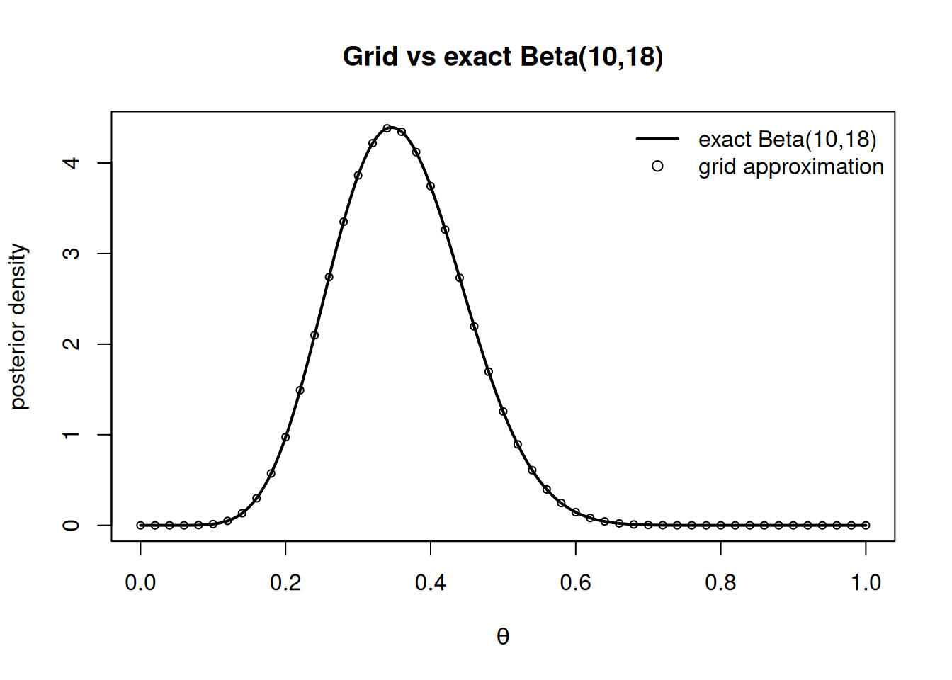
A correct grid approximation should sit on top of the exact \(\text{Beta}(10,18)\) curve.
exact <-dbeta(theta, 10, 18)grid_density <- post_grid / (theta[2] - theta[1]) # convert weights to density unitsplot(theta, exact, type ="l", lwd =2,xlab =expression(theta), ylab ="posterior density",main ="Grid vs exact Beta(10,18)")points(theta[seq(1, 1001, by =20)], grid_density[seq(1, 1001, by =20)],pch =1, cex =0.7)legend("topright", legend =c("exact Beta(10,18)", "grid approximation"),lty =c(1, NA), pch =c(NA, 1), lwd =c(2, NA), bty ="n")
Figure 1: Grid approximation (points) overlaid on the exact Beta(10,18) posterior (curve) for the bike proportion. Agreement confirms the grid is built correctly.
Step 3 — Sample posterior draws and summarize
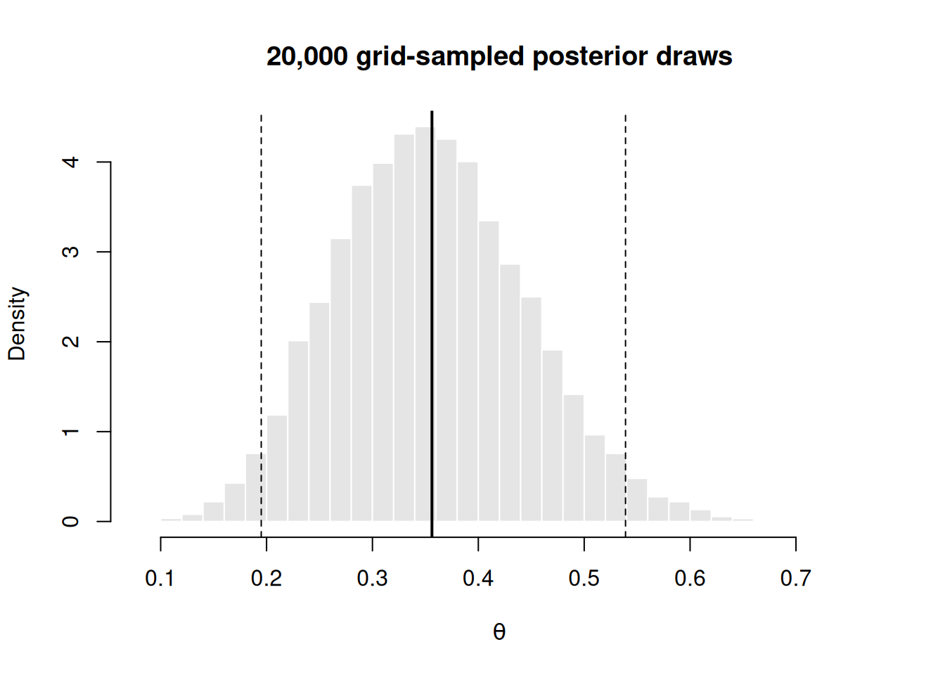
Draw from the grid with probabilities equal to the normalized weights, then summarize like any data. Seed first so the result reproduces.
Figure 2: Histogram of 20,000 grid-sampled posterior draws with the simulated mean (solid) and 95 percent credible interval (dashed).
Step 4 — Add a session record and render
End the report with a session record, then render the whole document.
sessionInfo()
R version 4.6.0 (2026-04-24)
Platform: x86_64-pc-linux-gnu
Running under: Ubuntu 24.04.4 LTS

Matrix products: default
BLAS:   /usr/lib/x86_64-linux-gnu/openblas-pthread/libblas.so.3
LAPACK: /usr/lib/x86_64-linux-gnu/openblas-pthread/libopenblasp-r0.3.26.so;  LAPACK version 3.12.0

locale:
 [1] LC_CTYPE=C.UTF-8       LC_NUMERIC=C           LC_TIME=C.UTF-8
 [4] LC_COLLATE=C.UTF-8     LC_MONETARY=C.UTF-8    LC_MESSAGES=C.UTF-8
 [7] LC_PAPER=C.UTF-8       LC_NAME=C              LC_ADDRESS=C
[10] LC_TELEPHONE=C         LC_MEASUREMENT=C.UTF-8 LC_IDENTIFICATION=C

time zone: UTC
tzcode source: system (glibc)

attached base packages:
[1] stats     graphics  grDevices utils     datasets  methods   base

loaded via a namespace (and not attached):
 [1] compiler_4.6.0  fastmap_1.2.0   cli_3.6.6       tools_4.6.0
 [5] htmltools_0.5.9 yaml_2.3.12     rmarkdown_2.31  knitr_1.51
 [9] jsonlite_2.0.0  xfun_0.58       digest_0.6.39   rlang_1.2.0
[13] evaluate_1.0.5
Render from the terminal (with R on PATH) or VS Code’s render button:
quarto render lab07.qmd
Verify
Your approximation is correct if the simulated mean matches the closed-form posterior mean. The closed form is \(\dfrac{\alpha + y}{\alpha + \beta + n} = \dfrac{10}{28} \approx 0.357\). Check it:
stopifnot(abs(closed_form - sim_mean) <0.01) # passes when grid + draws agree with the truth
Success criterion: the absolute difference is below 0.01, and the stopifnot does not error. If it errors, your grid is too coarse, your draw count is too small, or you forgot to normalize — revisit Step 1. (As a second check, your 95% credible interval should run roughly from about 0.20 to 0.53; say “credible interval,” never “confidence interval,” for a posterior.)
AI use note
Tool. A general coding assistant in your editor.
Purpose. Acceptable for scaffolding a chunk, decoding an R error, or drafting a caption — not for deciding what the posterior means.
Verification. Re-run any AI-suggested code and confirm the verify step still passes (|closed_form - simulated| < 0.01) and every random chunk is seeded. Disclose AI use per the course AI policy in the LMS. Unverifiable AI output does not go in a report you submit.
The graded deliverable, its rubric, point values, and due date live in the LMS — this lab page does not contain any of those. For grading specifics, the LMS (Blackboard) is authoritative.