Week 14 — Decisions & communication

Turning a posterior into a defensible recommendation — and saying it honestly

The week question

All term we have been answering what does the data tell us about the parameter? This week we ask the question that a stakeholder actually cares about: given everything our posterior says, what should we do — and how do we communicate that choice honestly, without pretending the uncertainty away?

Where we are and why this matters

We arrive here holding a full toolkit of posterior and predictive summaries from across the term. In the running bike-to-campus survey we began with a mild prior \(f(\theta) = \text{Beta}(2,2)\) on \(\theta\), the unknown proportion of students who bike to campus, observed \(y = 8\) bikers out of \(n = 24\) surveyed, and updated to the posterior \(f(\theta \mid y) = \text{Beta}(10, 18)\) with posterior mean \(10/28 \approx 0.357\) (Weeks 3–5). We learned to read a credible interval off that posterior, to push it forward into a posterior predictive distribution over future data (Week 6), and to build all of it by simulation (Week 7). We extended the same machinery to regression coefficients (Weeks 9–11) and to partial pooling across groups (Week 13).

Up to now every one of those summaries has been a description of belief. This week we cross a real line: from inference (what do I believe about \(\theta\)?) to decision (what action should I take?). Those are different activities. A posterior favors no particular action; a decision is a commitment in the world — buy the bike racks or do not, change the staffing or do not. Crossing that line well requires two new habits: state a decision rule that maps the posterior to an action (usually through a threshold), and communicate the result to people who will never see a Beta distribution, honestly and usably. Both are easy to get wrong, and getting them wrong is how good analyses turn into overconfident recommendations. This is also the conceptual home of your course project, which asks you to carry one question all the way from a prior to a communicated, uncertainty-aware decision.

Learning goals

By the end of this week you should be able to:

Convert a posterior into a decision through an explicit threshold rule, and state the rule before looking at the answer.
Compute and interpret a posterior probability of exceeding a threshold, e.g. \(P(\theta > c \mid y)\).
Distinguish four kinds of uncertainty — parameter, predictive, model, and decision — and say which one a given claim is about.
Recognize and avoid collapsing a full posterior to a single number that hides the uncertainty.
Communicate a recommendation to a non-technical audience honestly: the action, the evidence, the uncertainty, and what would change the call.

Core vocabulary

Decision rule — an explicit recipe that maps a posterior summary to an action (e.g. “recommend the investment if \(P(\theta > c \mid y)\) exceeds some agreed level”). It is chosen before seeing the number, so the data does not get to redefine what counts as success.
Decision threshold (\(c\)) — the substantively meaningful cutoff on the parameter that separates “act” from “do not act.” It comes from the problem, not from the data.
Posterior threshold probability — \(P(\theta > c \mid y)\), the posterior probability the parameter lies on the action side of the threshold; the area under the posterior beyond \(c\).
Parameter uncertainty — spread in the posterior \(f(\theta \mid y)\): we are unsure of the number.
Predictive uncertainty — spread in future data \(f(y_{\text{new}} \mid y)\): parameter uncertainty plus sampling variability (Week 6).
Model uncertainty — we are unsure the model itself is right (the likelihood form, the independence assumptions); not captured by any single posterior.
Decision uncertainty — we may make the wrong call even with a good model, because the threshold probability is not 0 or 1; the residual risk of acting (or not) under genuine uncertainty.

From inference to decision: the threshold move

A posterior does not, by itself, tell you what to do. To get an action you must supply something the data cannot: a threshold that says what level of the parameter matters, and a rule that says how confident you want to be before acting. Both belong to the decision-maker, not to the dataset.

Concretely, suppose the campus will install a new bike rack only if it is reasonably sure that more than a third of students bike — that is the level at which the racks pay for themselves. The substantive threshold is \(c = 0.33\). The decision rule is a statement like: recommend the racks if the posterior probability \(P(\theta > 0.33 \mid y)\) is high enough to act on. Notice what each piece does. The threshold \(c\) encodes what the world cares about. The confidence level encodes how cautious we want to be — how much decision uncertainty we are willing to carry. Neither is computed from the data; both are agreed in advance, in the open, so the analysis cannot quietly move the goalposts.

The quantity the data does supply is the posterior threshold probability \(P(\theta > c \mid y)\) — the area under the posterior to the right of \(c\), one line of base R for a Beta posterior. Crucially, \(P(\theta > c \mid y)\) is rarely 0 or 1. A value of, say, \(0.62\) does not mean “\(\theta\) is above the threshold.” It means given the model and data, there is a 62% posterior chance it is. The rule then decides whether 62% is enough. That gap between the probability and certainty is exactly decision uncertainty, and a good recommendation names it rather than rounding it away.

Four kinds of uncertainty (and which one you are talking about)

A decision can go wrong in four distinct ways, and clear communication depends on keeping them apart.

Parameter uncertainty — even with a perfect model, we do not know \(\theta\) exactly; the posterior has width. This is what a credible interval describes.
Predictive uncertainty — about future data, not the parameter. It stacks parameter uncertainty on top of sampling variability, so it is wider (Week 6). Use it when the decision is about what the next sample or season will look like.
Model uncertainty — our chosen data model (Binomial counts, a Poisson rate, a linear mean) might be the wrong story. No single posterior shows this; posterior predictive checks (Week 6) and sensitivity analysis (Week 5) are how we probe it. A confident posterior under a wrong model is confidently wrong.
Decision uncertainty — because \(P(\theta > c \mid y)\) sits strictly between 0 and 1, any call we make carries a chance of being the wrong call. This is irreducible without more data; the right response is to make it visible, not to hide it behind a crisp verdict.

The discipline is simple to state and hard to keep: every sentence in a recommendation is about exactly one of these. “We are 90% sure the true proportion exceeds a third” is parameter uncertainty; “next year’s survey will likely show between 5 and 13 bikers” is predictive; “this all assumes bikers were sampled independently” is model; “there’s a real chance we recommend the racks and turn out wrong” is decision uncertainty. Mixing them is the most common way technical results get garbled on the way to a decision-maker.

Communicating uncertainty to a non-technical audience

The goal of communication is not to dumb the analysis down; it is to transfer the honest shape of what you found to someone who will act on it. Three principles carry most of the weight.

Lead with the decision, then the evidence, then the uncertainty. A stakeholder needs the recommendation first (“we recommend installing the racks”), then the basis (“about a 3-in-5 posterior chance that more than a third of students bike”), then the caveat (“but this is not a sure thing, and here is what would change our mind”). Burying the recommendation under method loses the audience; omitting the uncertainty misleads them.

Translate probabilities into plain, comparable language — and keep the interval. “A 62% posterior probability” can become “a bit better than a coin flip in favor.” A credible interval of \(0.20\) to \(0.55\) can become “plausibly anywhere from a fifth to over half.” Never replace the interval with the point estimate alone: a recommendation that says “the proportion is 0.357, so build” has thrown away the very uncertainty that should temper the decision.

Name what would change the call. Honest communication is conditional: “if we surveyed 100 more students and the rate held, we’d be much more confident,” or “if bikers cluster by dorm, our independence assumption is shaky and the real uncertainty is wider.” This makes the decision uncertainty concrete rather than rhetorical, and invites better decisions instead of foreclosing them.

Worked example — a bike-rack decision threshold (recurring case)

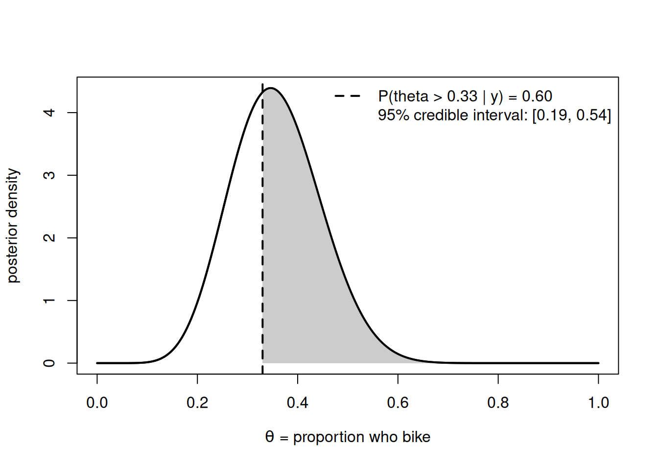
The facilities office will fund a new bike rack only if a meaningful share of students bike. They set the substantive threshold at \(c = 0.33\) (a third) and ask: what is the posterior probability that the true proportion exceeds a third, and what do we recommend? Our posterior is \(f(\theta \mid y) = \text{Beta}(10, 18)\). The honest summary is the shaded area beyond \(c\), plus the credible interval — never a lone point.

set.seed(1414)
c_thr <- 0.33
grid  <- seq(0, 1, length.out = 1000)
dens  <- dbeta(grid, 10, 18)

plot(grid, dens, type = "l", lwd = 2,
     main = "", xlab = expression(theta ~ "= proportion who bike"),
     ylab = "posterior density")

# Shade the action region theta > c
xr <- grid[grid >= c_thr]
yr <- dbeta(xr, 10, 18)
polygon(c(c_thr, xr, 1), c(0, yr, 0), col = "grey80", border = NA)
lines(grid, dens, lwd = 2)
abline(v = c_thr, lty = 2, lwd = 2)

# Posterior probability theta > c, and the 95% credible interval
p_exceed <- 1 - pbeta(c_thr, 10, 18)
ci       <- qbeta(c(0.025, 0.975), 10, 18)
legend("topright", bty = "n",
       legend = c(sprintf("P(theta > %.2f | y) = %.2f", c_thr, p_exceed),
                  sprintf("95%% credible interval: [%.2f, %.2f]", ci[1], ci[2])),
       lty = c(2, NA), lwd = c(2, NA))

A smooth posterior density curve for the bike proportion peaking near 0.36 and spanning roughly 0.15 to 0.6. A vertical dashed line at 0.33 marks the decision threshold, and the area under the curve to the right of that line is shaded, representing the posterior probability that the proportion exceeds a third, which is a bit over half of the total area. — Figure 1: The Beta(10,18) posterior for the bike-to-campus proportion, with the decision threshold c = 0.33 marked and the region θ > 0.33 shaded. The shaded area is the posterior probability that the true proportion exceeds a third — the number the recommendation rests on.

The shaded area is \(P(\theta > 0.33 \mid y) = 1 - \text{pbeta}(0.33, 10, 18) \approx 0.61\), and the 95% credible interval runs from about \(0.20\) to \(0.55\). Now apply a rule stated in advance. If facilities agreed to act only at a posterior probability of at least \(0.80\), then \(0.61\) does not clear the bar: the honest recommendation is “do not commit yet; the evidence leans toward a third or more (about a 3-in-5 chance) but falls short of the confidence we said we’d require, and the true rate could plausibly be as low as a fifth — a larger survey would sharpen this.” If the agreed bar were a more permissive \(0.50\), the same number clears it, and we would recommend the racks while still reporting the interval and the 39% chance of being wrong. The data did not change; the rule decided. That separation is the whole point.

Worked example — transfer: a clinic staffing decision (Gamma-Poisson)

Same logic, different model. A campus clinic models walk-ins per hour as \(\text{Poisson}(\lambda)\) and, from earlier work, holds a posterior \(f(\lambda \mid y) = \text{Gamma}(40, 8)\) (posterior mean \(40/8 = 5\) walk-ins/hour). Management will add an extra staffer only if the true rate exceeds \(c = 4.5\) per hour — below that, the existing staff cope. The decision quantity is the posterior probability \(P(\lambda > 4.5 \mid y)\), read as the area under the Gamma posterior beyond the threshold.

set.seed(1414)
c_thr <- 4.5
grid  <- seq(2, 9, length.out = 1000)
dens  <- dgamma(grid, shape = 40, rate = 8)

plot(grid, dens, type = "l", lwd = 2,
     main = "", xlab = expression(lambda ~ "= walk-ins per hour"),
     ylab = "posterior density")

xr <- grid[grid >= c_thr]
yr <- dgamma(xr, shape = 40, rate = 8)
polygon(c(c_thr, xr, max(grid)), c(0, yr, 0), col = "grey80", border = NA)
lines(grid, dens, lwd = 2)
abline(v = c_thr, lty = 2, lwd = 2)

p_exceed <- 1 - pgamma(c_thr, shape = 40, rate = 8)
ci       <- qgamma(c(0.025, 0.975), shape = 40, rate = 8)
legend("topleft", bty = "n",
       legend = c(sprintf("P(lambda > %.1f | y) = %.2f", c_thr, p_exceed),
                  sprintf("95%% credible interval: [%.2f, %.2f]", ci[1], ci[2])),
       lty = c(2, NA), lwd = c(2, NA))

A posterior density curve for the hourly walk-in rate peaking near 5 and spanning roughly 3.3 to 7. A vertical dashed line at 4.5 marks the staffing threshold, and the area under the curve to the right of the line is shaded, covering most of the distribution and representing a high posterior probability that the rate exceeds the cutoff. — Figure 2: The Gamma(40,8) posterior for the clinic walk-in rate, with the staffing threshold c = 4.5 per hour marked and the region λ > 4.5 shaded. The shaded area is the posterior probability the true rate exceeds the staffing cutoff.

Here \(P(\lambda > 4.5 \mid y) = 1 - \text{pgamma}(4.5, 40, 8) \approx 0.84\), with a 95% credible interval of roughly \(3.6\) to \(6.7\) walk-ins/hour. Under a pre-agreed action bar of \(0.80\), this clears it. The communicated version still carries the uncertainty: “add the staffer — there’s about an 84% chance the rate exceeds the cutoff; the rate is plausibly between about 3.6 and 6.7 per hour, and a roughly 1-in-6 chance the cutoff isn’t truly exceeded means we’d revisit after a month of new data.” Each clause is tagged to one kind of uncertainty — the interval is parameter uncertainty, the “1-in-6 chance of the wrong call” is decision uncertainty, and “revisit after new data” acknowledges that more information would shrink both.

A common mistake

Collapsing the full posterior to a single number and letting the data “prove” the decision.

The trap has two faces that often appear together. The first is premature collapse: reporting only the posterior mean — “the proportion is 0.357, so we should build” — and discarding the interval and the threshold probability. That hands the decision-maker a false crispness, hiding that the true proportion could plausibly be a fifth, which might flip the call. The second is the language of proof: “the data show we should install the racks.” Bayesian analysis never proves an action; it gives a posterior probability, and a separately chosen rule turns that into a revisable, fallible recommendation.

How to catch it: before you write a recommendation sentence, ask “have I stated a threshold and a rule that were fixed in advance, and have I reported the threshold probability AND an interval, not just a point?” If a single number is doing all the work, or if the word “prove” has snuck in, you have collapsed the posterior. The antidote is right there in the figures: the shaded area and the interval together, with the rule named out loud, so the uncertainty is on the page instead of behind it.

Interpretation guidance

A posterior threshold probability \(P(\theta > c \mid y)\) means exactly what it says: given this model and data, the posterior chance the parameter is on the action side of \(c\). It does not mean the parameter is above \(c\), it does not become a yes/no fact when it crosses some level, and it is not a long-run error rate (that would be a frequentist construction — keep “posterior probability” and “p-value” verbally distinct, as all term). It is a degree of belief, conditional on assumptions you should be willing to state.

A recommendation built from it is honest only when it carries its limits. The decision uncertainty — the chance of the wrong call — does not disappear because you committed to an action; it is the risk you decided to accept. Model uncertainty sits underneath everything: a tidy threshold probability from a misspecified model is precise but possibly wrong, which is why a write-up should name its key assumptions (here, that respondents were sampled independently and the proportion is stable over the period). And as always, pair the point with the interval and say which kind of quantity each sentence describes. The result you communicate should let a reasonable stakeholder disagree with your rule while trusting your numbers — that is the mark of a decision communicated well.

Practice (ungraded)

Use these to check your own understanding. No solutions are posted here.

Using the bike posterior \(\text{Beta}(10,18)\), compute \(P(\theta > 0.40 \mid y)\) with a single pbeta call. If the action bar were \(0.80\), would you recommend acting? Write the one-sentence recommendation, interval included.
A colleague writes: “Our posterior mean is 0.357, which proves more than a third of students bike.” Identify two separate things wrong with that sentence and rewrite it honestly.
For the clinic example, restate \(P(\lambda > 4.5 \mid y) \approx 0.84\) in plain language for a non-technical manager, in one sentence, without using the words “posterior” or “probability.”
Give one sentence each describing the bike decision in terms of (a) parameter uncertainty,
1. predictive uncertainty, (c) model uncertainty, and (d) decision uncertainty.
Two analysts use the same posterior but reach opposite recommendations. Without anyone making an arithmetic error, how is that possible — and what should each disclose so the disagreement is honest?

Reading guide

This week maps to Bayes Rules! Ch 8 — Posterior inference & prediction, read in its extended sense as the decision chapter. Earlier (Week 6) we used Ch 8 for the predictive strand; now return to its treatment of using the posterior to test claims and act on them. Read the chapter’s posterior hypothesis material as the engine behind our threshold probability \(P(\theta > c \mid y)\): where the book frames it as evaluating a hypothesis about \(\theta\), we extend the same area-under-the-posterior idea into a stated decision rule and a communicated recommendation. The chapter’s emphasis on reporting a posterior probability rather than a verdict is precisely the habit this week formalizes. Hold the running bike example beside the book’s worked case so the structure — threshold, threshold probability, interval, honest statement — transfers even though the numbers differ. We adapt the chapter’s concepts in the course’s own framing and synthetic examples; the text is used under CC BY-NC-SA 4.0.

Public vs. graded

These notes and the ungraded practice above are public and for learning only: no answer keys are posted here, and nothing on this page sets graded prompts, rubric values, point values, or due dates — including for the course project. For anything that counts toward your grade — project specifics, deliverables, deadlines — the LMS (Blackboard) is authoritative. Where this page and the LMS differ, the LMS governs.

Looking ahead

You now have the full arc: prior, posterior, prediction, and a decision communicated under honest uncertainty. Next week, Week 15 — Project workshop & synthesis, we put it all to work — workshopping your project so that one question travels from a prior all the way to a recommendation a stakeholder could act on. See Week 15 — Project workshop & synthesis.