Complete pooling, no pooling, partial pooling, and why estimates shrink
Mathematical goal
This week we write down the simplest hierarchical model and use it to make precise an idea that has been hovering since the first weeks: when we estimate many related quantities at once — the mean exam score in each of several sections of the same course — we do not have to choose between treating the sections as identical and treating them as unrelated. A hierarchical model lets each section have its own mean while also declaring that those means are themselves draws from a shared population distribution. The mathematical payoff is partial pooling: each group’s estimate becomes a weighted average of its own data and the overall mean, and the weights follow a clean formula. By the end you should be able to state the two-level model, write the partial-pooled estimate as that weighted average, and explain — symbolically and on a numeric instance — why small or noisy groups shrink more.
The week question
When we estimate a separate mean for each of several related groups, how much should each group’s estimate be allowed to lean on its own data versus borrow strength from the other groups — and what does the math say that “borrowing” looks like?
Where we are and why this matters
All term we have built up the posterior-as-distribution view: a parameter \(\theta\) is not a single number to be pinned down but a quantity we describe with a full distribution \(f(\theta \mid y)\), summarized by a point estimate and a credible interval. We also learned (Weeks 3–5) to treat the prior as information — a Beta(2,2) on the bike-to-campus proportion encoded a mild starting belief, and the data reshaped it through \(f(\theta \mid y) \propto L(\theta \mid y)\, f(\theta)\).
This week both ideas scale up to many parameters at once. Instead of one proportion or one mean, imagine the mean exam score \(\theta_j\) in section \(j\) of a multi-section course. We now have a posterior over each\(\theta_j\), and — this is the new move — the prior on the \(\theta_j\) is not something we type in by hand. It is estimated from the groups themselves: the sections tell us what a “typical section mean” looks like, and that shared population distribution acts as a data-driven prior that pulls each group’s estimate toward the center. That is why partial pooling matters: it is the principled middle ground between pretending all sections are the same and pretending they have nothing to do with each other, and it usually predicts new data better than either extreme.
Notation
This week’s notation extends the fixed course ledger to indexed groups. The table is the working vocabulary the derivation manipulates; read it before the algebra.
Symbol
Meaning
\(j\)
a group index, \(j = 1, \dots, J\) (here, a course section)
\(J\)
the number of groups
\(n_j\)
the number of observations in group \(j\)
\(\theta_j\)
the unknown mean of group \(j\) — its own parameter
\(\bar y_j\)
the observed sample mean in group \(j\) (the no-pooling estimate)
\(\mu\)
the population (overall) mean — the center the group means cluster around
\(\tau^2\)
the between-group variance — how spread out the \(\theta_j\) are around \(\mu\)
\(\sigma^2\)
the within-group variance — noise of individual observations within a section (assumed known/common here)
\(f(\theta_j \mid y)\)
the posterior for group \(j\)’s mean
One naming caution carried from earlier weeks: \(\sigma^2\) is a variance, written \(N(\mu,\sigma^2)\) in the course’s mean–variance convention for the Normal; we never silently switch it for a standard deviation in a formula.
Conceptual setup
Before any algebra, set up the assumptions and recall the three ways one could handle grouped data. Assume we observe \(J\) sections; in section \(j\) we have \(n_j\) scores with sample mean \(\bar y_j\), and within any section a single score is Normal around that section’s true mean \(\theta_j\) with known common variance \(\sigma^2\).
There are three modeling stances:
Complete pooling. Assume every section has the same mean: \(\theta_1 = \dots = \theta_J = \mu\). Throw all scores into one pile and estimate a single number. This ignores real differences between sections — it under-fits.
No pooling. Assume the section means are unrelated; estimate each \(\theta_j\) from its own data alone, so the estimate is just \(\bar y_j\). Small or noisy sections get wild, unstable estimates because a handful of scores drives them — it over-fits.
Partial pooling. The hierarchical compromise: assume the section means are different but related, all drawn from one population distribution. Each estimate is pulled part way from its own \(\bar y_j\) toward the overall mean \(\mu\). Recall this is exactly the “prior as information” idea — but the prior is learned from the groups.
The hierarchical model is the formal statement of the third stance, and partial pooling is what its posterior does automatically.
The two-level model statement
A hierarchical model is built in levels. Level one is the data model — how individual scores relate to their section mean. Level two is the prior on the section means, which is where the sharing happens.
Read level two carefully: it says the section means \(\theta_j\) are themselves random draws from a shared \(N(\mu, \tau^2)\). That shared distribution is the population of sections. Its center \(\mu\) is “the typical section mean,” and its spread \(\tau\) controls how different sections are allowed to be. When \(\tau\) is large, sections are very different and level two barely constrains them (we approach no pooling); when \(\tau \to 0\), all sections collapse onto \(\mu\) (we approach complete pooling). Partial pooling lives in between, and the data decide where.
(A fully Bayesian treatment also puts priors on \(\mu\), \(\tau\), and \(\sigma\) — a third level — and estimates them too; at this introductory level we hold \(\sigma^2\) and \(\tau^2\) fixed so the shrinkage formula stays in closed form, and flag the rest as the natural next step.)
The shrinkage formula
Take \(\sigma^2\) and \(\tau^2\) as known and \(\mu\) as the overall center. With a Normal data model and a Normal level-two prior, the per-group posterior follows the Normal–Normal conjugate update — our same posterior \(\propto\) likelihood \(\times\) prior reflex, specialized to the Normal family: a Normal prior combined with Normal data yields a Normal posterior whose mean is a precision-weighted average of the two. Applied to each group, the prior on \(\theta_j\) is \(N(\mu, \tau^2)\), and the data contribute the section mean \(\bar y_j\), which behaves like one observation with variance \(\sigma^2/n_j\). The posterior mean of \(\theta_j\) is the precision-weighted average of the two:
The weight \(\lambda_j\) on the group’s own data runs between 0 and 1. Define the shrinkage factor as \(1 - \lambda_j\), the weight placed on the overall mean. Stare at \(\lambda_j\):
It grows with \(n_j\) — a section with many scores trusts its own \(\bar y_j\), so \(\lambda_j \to 1\) and it barely shrinks.
It shrinks with \(\sigma^2\) — noisier within-section data (\(\sigma^2\) large) means the group’s own mean is less reliable, so more weight goes to \(\mu\).
It grows with \(\tau^2\) — if sections are genuinely very spread out, pulling toward the center is less justified.
So small, noisy groups shrink most; large, clean groups shrink least. That single sentence is the whole intuition, and the formula above is the proof.
Worked examples
We work a symbolic case (the two-level statement and the weighted-average estimate) and a numeric instance you can re-run, both on the recurring exam-scores-across-sections setting; then a transfer case in a new context.
Worked example — exam scores across sections (symbolic, then numeric)
This is the recurring hierarchical case: \(\theta_j\) is the true mean exam score in section \(j\).
Symbolic. Write the model and the partial-pooled estimate:
Contrast the three estimates symbolically: complete pooling reports \(\mu\) for every section (\(\lambda_j = 0\) for all \(j\)), no pooling reports \(\bar y_j\) (\(\lambda_j = 1\)), and partial pooling slides between them with \(\lambda_j\) set by the data.
Numeric instance. Take \(J = 5\) sections (label them A–E) with within-section noise \(\sigma = 10\) and a modest between-section spread \(\tau = 6\). The sections have sizes \(n = (8, 30, 12, 6, 20)\) — deliberately mixing a few small sections with larger ones. We simulate scores from synthetic section truths and compute, for each section, its no-pooling mean \(\bar y_j\), the overall (complete-pooling) mean \(\mu\), and the partial-pooled estimate. With the seed below the section means come out near
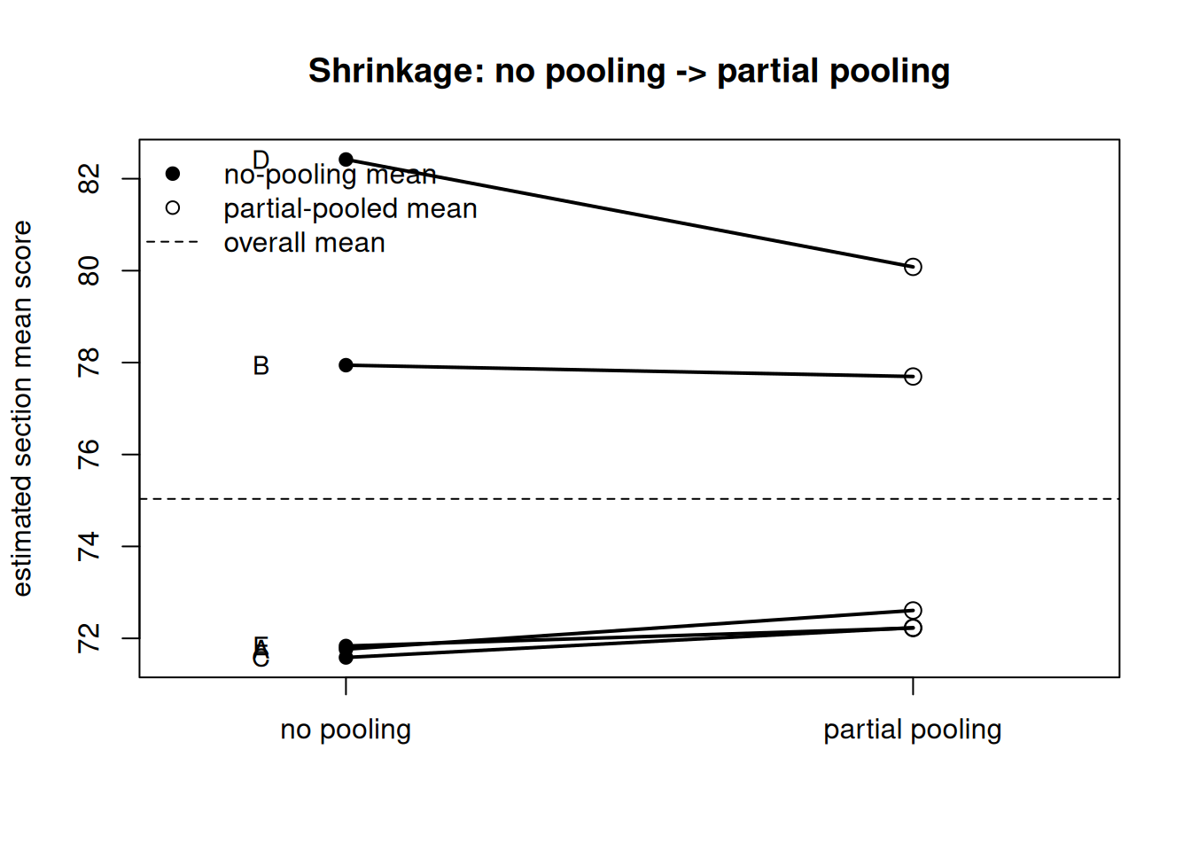
and the partial-pooled estimates near \((72.6,\ 77.7,\ 72.2,\ 80.1,\ 72.2)\). Notice section D: it is the smallest (\(n_4 = 6\)) and the most extreme (\(\bar y_4 \approx 82.4\)), and it moves the most — about \(2.3\) points toward the center — while the largest section B (\(n_2 = 30\)) barely moves (\(\approx 0.25\) points). The figure makes the shrinkage visible as line segments connecting each no-pooling estimate to its pulled-in partner.
Figure 1: No-pooling section means (left column) connected by segments to their partial-pooled (shrunken) estimates (right column) for five synthetic sections, with the overall mean shown as a horizontal reference. The smallest, most extreme section (D) is pulled the furthest toward the center; the largest section (B) barely moves.
The printed estimates confirm the picture: every partial-pooled value sits between its \(\bar y_j\) and the overall mean \(\mu \approx 75\), and the smaller the section, the larger the pull.
  section  n no_pooling lambda partial_pooled overall
1       A  8      71.76   0.74          72.61   75.03
2       B 30      77.94   0.92          77.70   75.03
3       C 12      71.58   0.81          72.23   75.03
4       D  6      82.42   0.68          80.08   75.03
5       E 20      71.83   0.88          72.22   75.03
Worked example — transfer case (clinic wait times across branches)
To show this is about structure, transfer it to the secondary recurring counts setting, recast as means. A health system has \(J = 3\) clinic branches; we record the mean wait time (minutes) at each. The smallest branch logged only \(n_1 = 5\) visits with a noisy \(\bar y_1 = 41\) minutes; the busy branches logged \(n_2 = 60\) (\(\bar y_2 = 24\)) and \(n_3 = 80\) (\(\bar y_3 = 22\)), with overall mean \(\mu \approx 24\). Apply the same level-two idea: the tiny branch’s \(41\) is the least reliable, so its partial-pooled estimate is pulled hard toward \(\mu \approx 24\), landing well below \(41\), while the two large branches barely move. We would report each branch as a partial-pooled mean with a credible interval, never a bare \(\bar y_j\) — and we would explicitly not claim the small branch’s raw \(41\) is its honest estimate. The story changed; the shrinkage math did not.
A convention warning
Two conventions and one caution cause most of the avoidable errors here.
Partial pooling is not “averaging away” real differences. Shrinkage does not force the groups to the same value — that is complete pooling. The \(\theta_j\) stay distinct; they are merely pulled part way toward the center by an amount the data set through \(\lambda_j\). A large, clean group keeps almost all of its own signal. Saying “partial pooling erases group differences” is the central misconception of the week; the convention is that shrinkage regularizes, it does not homogenize.
Shrinkage depends on group size and variance, not on how far the group looks. It is tempting to think the most extreme-looking group is shrunk most “because it’s an outlier.” The formula says otherwise: the amount of pull is governed by \(n_j\), \(\sigma^2\), and \(\tau^2\) through \(\lambda_j\) — a small/noisy group shrinks more even if it is near the center. The visible distance moved is (shrinkage factor) \(\times\) (gap to \(\mu\)), so a small and extreme group like section D moves most, but smallness, not extremeness, is the cause.
Credible, not confidence; and report an interval. Each \(\hat\theta_j^{\text{PP}}\) is a posterior mean and must be paired with a 95% credible interval for \(\theta_j\) — a posterior probability statement about that group’s mean — never reported as a bare point, and never called a confidence interval. Partial-pooled intervals are also typically narrower than no-pooling intervals for small groups, because the group borrows strength.
Practice (ungraded)
Use these to practice the ideas; no answer keys are posted here.
Write the two-level model for “average daily steps in each of four dorms,” naming what each of \(\theta_j\), \(\mu\), \(\tau^2\), and \(\sigma^2\) means in that context.
Two sections have the same noisy data (\(\sigma^2\) equal) but \(n = 5\) versus \(n = 50\). Which one shrinks more toward the overall mean, and why? Compute \(\lambda_j\) for each if \(\sigma = 10\) and \(\tau = 6\).
In the worked numeric instance, section B barely moved while section D moved a lot. Explain in one sentence each which property of the section drives that.
A classmate says “partial pooling just replaces every section with the overall average.” Correct them in two sentences using the words shrinkage and \(\lambda_j\).
As \(\tau \to 0\) and then as \(\tau \to \infty\), which of the three pooling stances does partial pooling approach? Tie your answer to the formula for \(\lambda_j\).
Formula-verification status
These formulas are prepared as evidence but NOT yet human/source verified (verified: false); see the notation ledger. The course math gate is blocked pending sign-off. In particular, the two-level model statement, the partial-pooled posterior mean \(\lambda_j\,\bar y_j + (1-\lambda_j)\,\mu\) with \(\lambda_j = (n_j/\sigma^2)/(n_j/\sigma^2 + 1/\tau^2)\), and the limiting behavior as \(\tau \to 0\) and \(\tau \to \infty\) are staged here as derivation evidence. They should be treated as provisional until the math gate is cleared and a reviewer’s sign-off is recorded against the ledger.
Public vs. graded
This is a public, ungraded study note: no answer keys are posted here. Worked examples, practice prompts, and figures are for learning, not for credit. Anything graded — homework prompts and their keys, weights, rubrics, point values, and due dates — lives in the LMS (Blackboard), which is authoritative for all of it. If this page and the LMS ever disagree, follow the LMS.
Looking ahead
Next week (Week 14 — Decisions & communication) we turn from building models to acting on and explaining them: how to summarize a posterior for a decision and communicate uncertainty to a non-technical audience. See Week 14 — Decisions & communication.