Lab 13 — Partial pooling

Compute and visualize shrinkage on synthetic section data, then check it against the closed form

Purpose. This lab is the hands-on companion to Week 13 — Hierarchical models. There you wrote the two-level model and the partial-pooling formula \(\hat\theta_j^{\text{PP}} = \lambda_j\,\bar y_j + (1-\lambda_j)\,\mu\). Here you produce the three estimates — no pooling, complete pooling, partial pooling — from seeded synthetic section data, visualize the shrinkage, and verify your simulated partial-pooled mean matches the closed-form value.

Goal

Compare no-pooling, complete-pooling, and partial-pooling estimates on synthetic section data and visualize shrinkage. By the end you will have (1) the three estimates per section in a table, (2) a shrinkage plot connecting each section’s no-pooling mean to its partial-pooled mean, and (3) a numeric check that the closed-form partial-pooled mean agrees with a simulated posterior mean — all reproduced from a seeded, re-runnable .qmd.

Setup

First, make sure your local toolchain is ready: R, VS Code, and Quarto, following the R + VS Code + Quarto setup page. Then, create a new file named lab-13.qmd, paste the chunks below in order, and render top to bottom. Every chunk uses base R only — no add-on packages — so it runs on a clean install. Seeds are fixed so your numbers match the text.

Steps

Step 1 — Simulate synthetic section data

We invent five course sections of mixed size with known within-section noise sigma and a known between-section spread tau. Keeping the truth known lets you later check that partial pooling behaves the way the formula predicts. These are the same settings as the Week 13 note.

set.seed(1313)
sigma <- 10        # within-section sd (known)
tau   <- 6         # between-section sd (known)
sizes <- c(8, 30, 12, 6, 20)
labels <- c("A", "B", "C", "D", "E")
true_means <- c(70, 78, 73, 84, 76)   # synthetic section truths

# store each section's raw scores in a list
scores <- vector("list", length(sizes))
for (j in seq_along(sizes)) scores[[j]] <- rnorm(sizes[j], true_means[j], sigma)
sapply(scores, length)                 # confirm the section sizes

[1]  8 30 12  6 20

Step 2 — The three estimates

Compute the no-pooling mean (each section’s own average), the complete-pooling mean (one overall average), and the partial-pooled mean (the precision-weighted blend from Week 13).

ybar <- sapply(scores, mean)                       # no pooling
grand <- sum(sizes * ybar) / sum(sizes)            # complete pooling (overall mean)
lambda <- (sizes / sigma^2) / (sizes / sigma^2 + 1 / tau^2)
pp <- lambda * ybar + (1 - lambda) * grand         # partial pooling

data.frame(section = labels, n = sizes,
           no_pooling = round(ybar, 2),
           complete_pooling = round(grand, 2),
           lambda = round(lambda, 2),
           partial_pooled = round(pp, 2))

  section  n no_pooling complete_pooling lambda partial_pooled
1       A  8      71.76            75.03   0.74          72.61
2       B 30      77.94            75.03   0.92          77.70
3       C 12      71.58            75.03   0.81          72.23
4       D  6      82.42            75.03   0.68          80.08
5       E 20      71.83            75.03   0.88          72.22

Read the table: every partial_pooled value sits between its no_pooling value and the complete_pooling overall mean, and lambda (the weight on the section’s own data) is smallest for the smallest sections.

Step 3 — Visualize the shrinkage

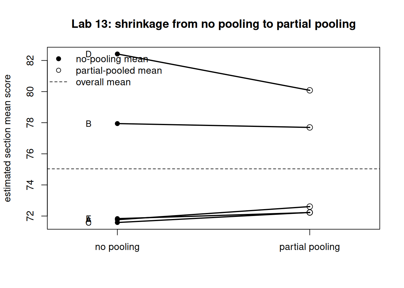
Draw the shrinkage plot: each section’s no-pooling mean on the left, its partial-pooled mean on the right, joined by a segment, with the overall mean as a dashed reference. Steeper segments are sections that shrank more.

plot(NA, xlim = c(0.7, 2.3), ylim = range(c(ybar, pp, grand)),
     xaxt = "n", xlab = "", ylab = "estimated section mean score",
     main = "Lab 13: shrinkage from no pooling to partial pooling")
axis(1, at = c(1, 2), labels = c("no pooling", "partial pooling"))
abline(h = grand, lty = 2, lwd = 1)
for (j in seq_along(sizes)) {
  segments(1, ybar[j], 2, pp[j], lwd = 2)
  points(1, ybar[j], pch = 19)
  points(2, pp[j], pch = 1, cex = 1.3)
  text(0.85, ybar[j], labels[j], cex = 0.9)
}
legend("topleft",
       legend = c("no-pooling mean", "partial-pooled mean", "overall mean"),
       pch = c(19, 1, NA), lty = c(NA, NA, 2), lwd = c(NA, NA, 1), bty = "n")

Figure 1: Shrinkage plot for five synthetic sections: no-pooling means (left) connected to partial-pooled means (right), with the overall mean dashed. Small sections shrink more than large ones.

Step 4 — Check the closed form by simulation

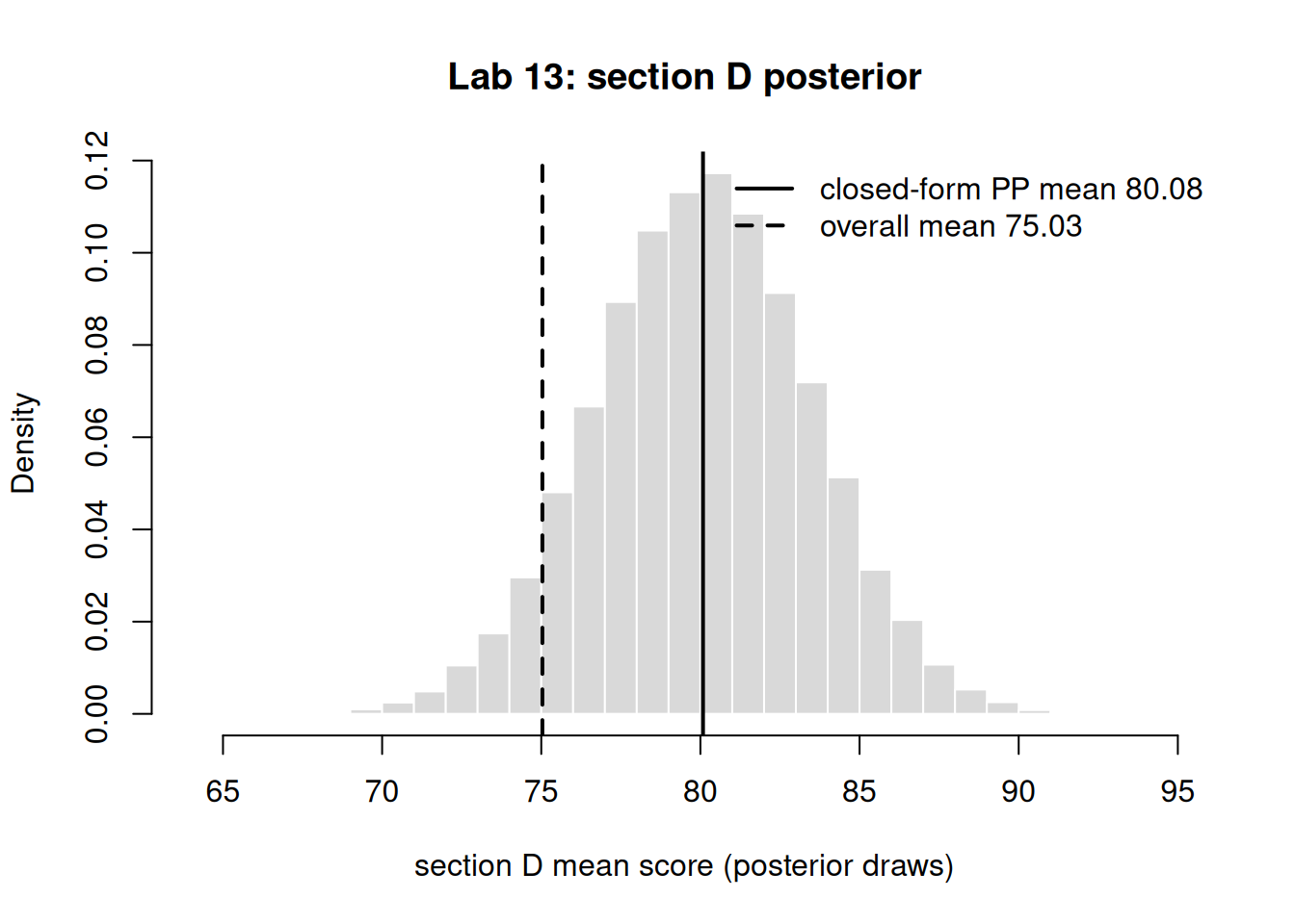
For one section, build the posterior for \(\theta_j\) directly: with a Normal data model and a Normal \(N(\mu, \tau^2)\) level-two prior (known variances), the posterior for \(\theta_j\) is Normal with mean equal to the partial-pooled value and precision \(n_j/\sigma^2 + 1/\tau^2\). Simulate from that Normal and confirm the simulated mean matches the closed-form pp from Step 2. We use the small section D, where shrinkage is largest.

jD <- 4                                            # section D
post_prec <- sizes[jD] / sigma^2 + 1 / tau^2       # posterior precision
post_sd   <- sqrt(1 / post_prec)
post_mean <- pp[jD]                                # = closed-form partial-pooled mean

set.seed(1313)
draws <- rnorm(50000, post_mean, post_sd)
hist(draws, breaks = 40, freq = FALSE, col = "grey85", border = "white",
     xlab = "section D mean score (posterior draws)",
     main = "Lab 13: section D posterior")
abline(v = post_mean, lwd = 2)
abline(v = grand, lwd = 2, lty = 2)
legend("topright",
       legend = c(sprintf("closed-form PP mean %.2f", post_mean),
                  sprintf("overall mean %.2f", grand)),
       lty = c(1, 2), lwd = 2, bty = "n")

c(sim_mean = mean(draws), closed_form = post_mean,
  abs_diff = abs(mean(draws) - post_mean))

    sim_mean  closed_form     abs_diff 
80.076117278 80.081730019  0.005612741 

Figure 2: Simulated posterior for section D’s mean (Normal with the closed-form partial-pooled mean and precision n/sigma^2 + 1/tau^2), with the closed-form mean and overall mean marked. The simulated mean lands on the closed-form value.

Illustrative — the same model with the course packages

The block below is illustrative only — it runs with the course packages (rstanarm, bayesrules) and is not executed here. It shows the genuine hierarchical fit you would run once those packages are installed; it estimates \(\mu\), \(\tau\), and \(\sigma\) jointly and returns a posterior for every section mean.

# illustrative — runs with the course packages, not executed in this lab
library(rstanarm)
long <- data.frame(
  score   = unlist(scores),
  section = factor(rep(labels, sizes))
)
model <- stan_glmer(
  score ~ 1 + (1 | section),         # varying intercept = partial pooling
  data   = long,
  family = gaussian,
  seed   = 1313
)
# partial-pooled section means with credible intervals:
coef(model)$section
posterior_interval(model, prob = 0.95)

Verify

Your work is on track if all three hold:

1. In Step 2, every partial_pooled value lies between that section’s no_pooling value and the overall complete_pooling mean — partial pooling never overshoots either extreme.
2. The smallest section (D, \(n = 6\)) has the smallest lambda and moves the most toward the overall mean, while the largest section (B, \(n = 30\)) has the largest lambda and barely moves.
3. In Step 4, the simulated posterior mean matches the closed-form partial-pooled mean. (Concrete success criterion: abs(mean(draws) - post_mean) < 0.1.)

If any check fails, see the next section.

When it breaks

• object 'pp' not found in Step 3 or 4 — Step 2 did not run; chunks share state only when executed in sequence. Fix by rendering the whole .qmd top to bottom.
• Numbers don’t match the text — confirm set.seed(1313) ran in the same chunk before the random draw; a missing or moved seed is the most common error here. Troubleshoot by re-rendering from a clean session.
• A partial-pooled value lands outside the no-pooling/overall range — you likely swapped lambda and 1 - lambda; the weight lambda multiplies ybar (the section’s own data), not the overall mean. Re-check Step 2.
• If the Step 4 difference is large — verify post_prec uses sigma^2 and tau^2 (variances, not sds) and that jD <- 4; a mismatched index compares the wrong section.

AI use note

Tool	Purpose	Verification
LLM assistant (e.g. Claude)	Explain an R error message or suggest a base-R plotting tweak for the shrinkage figure	Re-render the chunk yourself; confirm the table, figure, and the Step 4 difference satisfy the Verify criteria before trusting any AI-suggested edit.

Disclose AI assistance per the syllabus. AI may help you understand code; the runnable result and its interpretation must be your own and must pass the Verify checks.

See also

• Week 13 — Hierarchical models
• R + VS Code + Quarto setup
• Notation glossary

---

The graded deliverable, its rubric, point values, and due date live in the LMS (Blackboard), which is authoritative. None of those are posted here; this lab is the public, ungraded practice path.