Week 11 — Model checking & comparison

Asking whether a fitted model could have produced our data, and how to choose between rivals

The week question

For three weeks we have built regression models and read their coefficients. This week we cross-examine them instead: if a fitted model is right, could it have produced data that looks like ours — and when two models both seem to fit, how do we choose the one that will predict well rather than the one that merely memorized the data we already have?

Where we are and why this matters

We arrive here with two tools already in hand. From Weeks 9 and 10 we have the regression models: the study-hours/exam-score line \(y_i = \beta_0 + \beta_1 x_i + \varepsilon_i\) with a posterior over the coefficients, and its extensions to several predictors and to binary outcomes. From Week 6 we have the posterior predictive distribution \(f(y_{\text{new}} \mid y)\) — the data model averaged over the posterior, simulated with the two-step draw (first draw \(\theta\) from the posterior, then draw data given \(\theta\)). This week is where those two strands meet. We point the posterior predictive machinery back at our own data to interrogate the regression we just fit.

Why does this matter enough to spend a week on it? Because fitting a model is the easy part. R will happily fit a line, a curve, or a ten-predictor monster to any dataset, and every one of them will report tidy coefficient summaries. None of that tells you whether the model is adequate — whether it captures the features of the data you care about — or whether it will generalize to data it has not seen. A model that hugs the training data perfectly can be worse than a simpler one at predicting tomorrow. The discipline of checking a model and comparing models honestly is what separates a fit from an answer you can trust. That discipline is the heart of outcome O8 (use posterior predictive thinking to check model adequacy) and connects to O11 (distinguish parameter, predictive, model, and model-choice uncertainty).

Learning goals

By the end of this week you should be able to:

Run a posterior predictive check (PPC) on a regression model: simulate replicated datasets from the fitted model and compare them, on a chosen summary, to the data you actually observed.
Choose test quantities (summaries) that target features you care about, and read where the observed value sits in the replicated crowd.
Explain the difference between in-sample fit and out-of-sample predictive performance, and why the first can lie about the second.
Describe overfitting in plain terms and say why a more complex model is not automatically better.
Compare candidate models using predictive thinking, and state honestly what a comparison does and does not establish.
Apply the maxim “all models are wrong, but some are useful” as a working stance, not a shrug.

Core vocabulary

Posterior predictive check (PPC) — comparing observed data (or a summary of it) to data replicated from the fitted model, to judge whether the model could plausibly have produced what you saw.
Replicated dataset (\(y^{\text{rep}}\)) — a synthetic dataset of the same size and shape as your real data, drawn from the posterior predictive distribution as if the model were true.
Test quantity (summary) — a number computed from a dataset that you use for checking: a mean, a spread, a maximum, the count of values above a threshold, the size of the largest residual.
In-sample fit — how well a model matches the very data it was trained on. Always looks better for more complex models; a weak guide to prediction.
Out-of-sample predictive performance — how well a model predicts new data it did not see. The honest target.
Overfitting — chasing the noise in the training data with extra flexibility, buying in-sample fit at the cost of out-of-sample prediction.
Model comparison — judging candidate models against each other, ideally on predictive performance, not on which one fits the training data most tightly.

Posterior predictive checks for regression

In Week 6 we checked a single-proportion model by replicating counts. The move for regression is the same idea with a richer data object: a whole dataset of \((x_i, y_i)\) pairs rather than one count. The recipe does not change.

Fit the regression and get the posterior over \((\beta_0, \beta_1, \sigma)\).
Replicate. Draw a parameter vector from the posterior; at those parameter values, generate a new outcome \(y_i^{\text{rep}}\) for each observed \(x_i\) from the data model \(y_i^{\text{rep}} \sim N(\beta_0 + \beta_1 x_i,\ \sigma^2)\). That gives one replicated dataset the same size as yours. Repeat many times.
Summarize. Compute a test quantity on each replicated dataset and on the observed dataset.
Compare. Does the observed summary look like a typical draw from the replicates, or does it sit out in a tail?

The key insight is that a regression model is a generative story: “outcomes scatter Normally around a straight line with constant spread.” A PPC asks whether that story, run forward, produces datasets that look like the one in front of you. The story can be wrong in many ways — the relationship might curve, the spread might grow with \(x\), there might be outliers the Normal tails cannot accommodate — and each kind of wrongness shows up as a different test quantity landing in the tail. That is why a PPC is less a single verdict than a set of targeted questions: you check the features you care about.

A natural and powerful family of test quantities for regression is built from residuals — the gaps between observed outcomes and the line. If the model is right, the observed residuals should look like the residuals of the replicated datasets. A residual pattern that the model never reproduces (say, systematically larger residuals at large \(x\)) is a flag that the constant-spread or straight-line assumption is failing.

In-sample fit versus out-of-sample prediction

Here is the trap the whole week is built to disarm. Suppose you fit two models to the study-hours data: a straight line, and a wiggly high-degree polynomial. The polynomial will pass closer to every observed point — its in-sample fit is better, guaranteed, because it has more freedom to bend toward the data. If “fits the data better” meant “is a better model,” you would always pick the most flexible thing available. You would always be wrong.

The reason is that your data is signal plus noise. A straight-line relationship (signal) is buried in measurement error and the thousand small causes we do not model (noise). A flexible model cannot tell signal from noise; given enough freedom it fits both, bending to chase random wiggles that will not repeat in new data. When new data arrives — drawn from the same signal but fresh noise — the overfit model’s contortions point the wrong way, and it predicts worse than the humble line. This is overfitting: paying in future prediction for the illusion of present fit.

The honest target is therefore out-of-sample predictive performance: how well the model predicts data it did not train on. We cannot read this off the training fit, which is exactly why in-sample measures (like raw fit-to-the-data) systematically flatter complex models. Practical Bayesian model comparison estimates out-of-sample performance — for example by scoring how well each model predicts held-out observations, or by approximating that with cross-validation-style measures. The numerical machinery (the course packages compute predictive scores for you) is less important here than the principle: compare models on their ability to predict the unseen, not to memorize the seen.

Comparing candidate models without overfitting

Putting checking and prediction together gives a workable comparison stance for this course.

First, a model must pass its predictive checks to be a candidate at all. If a model cannot reproduce features of your data that matter, no comparison score rescues it. Checking is a screening gate.

Second, among models that pass, prefer the one that predicts new data best, not the one with the tightest training fit. When two models predict comparably, prefer the simpler one — fewer predictors, less flexibility — because it is less prone to overfitting and easier to interpret and trust. This is a Bayesian echo of parsimony: extra complexity must earn its place by improving out-of-sample prediction, not merely by hugging the data.

Third, report the comparison with its uncertainty. A predictive score is itself estimated from finite data and carries error; a small difference between two models’ scores may not be meaningful. Just as we never report a coefficient without a credible interval, we never report “Model A beats Model B” without asking whether the margin exceeds its own uncertainty. This is the model-choice flavor of uncertainty named in O11: even our choice between models is uncertain.

Worked example — a PPC on the study-hours model that PASSES (recurring case)

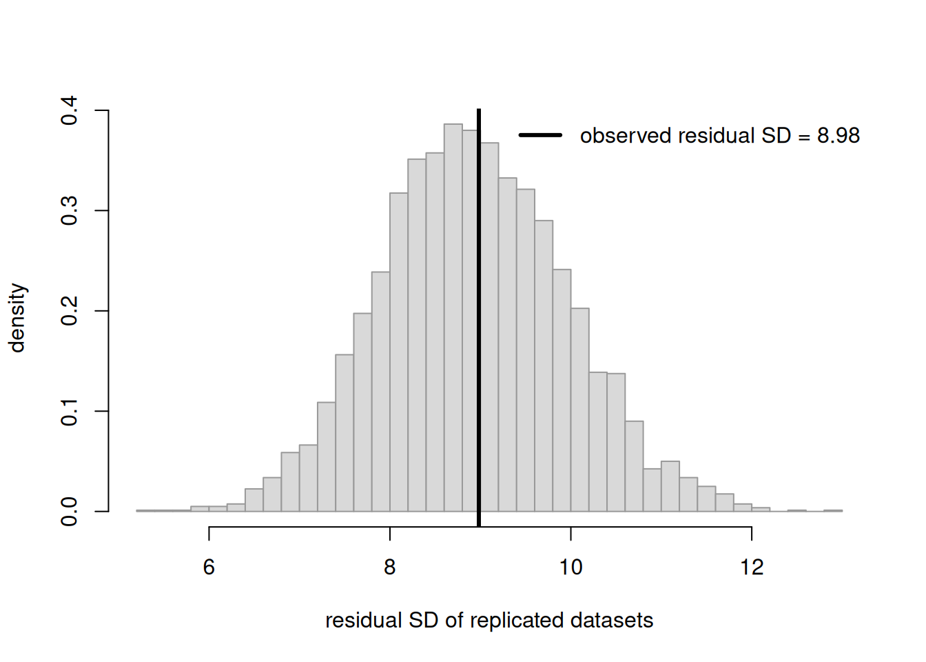
Take the Week 9 strand: study hours \(x\) predicting exam score \(y\), modeled as \(y_i \sim N(\beta_0 + \beta_1 x_i,\ \sigma^2)\). We generate synthetic data from a genuinely linear process, fit the line, then run a posterior predictive check using a sensible test quantity — the standard deviation of the residuals (does the model reproduce the observed scatter around the line?). Because the data really is linear with constant spread, the check should pass: the observed residual spread should land in the middle of the replicated spreads. All randomness is seeded.

set.seed(1111)
n  <- 40
x  <- runif(n, 0, 12)                       # study hours
y  <- 55 + 2.6 * x + rnorm(n, 0, 8)         # truly linear, constant spread

fit  <- lm(y ~ x)                           # fit the straight line
b    <- coef(fit); s <- summary(fit)$sigma  # plug-in params for replication
obs_sd <- sd(resid(fit))                    # observed test quantity

# Replicate datasets at the fitted params; recompute residual SD each time
R <- 4000
rep_sd <- numeric(R)
for (r in 1:R) {
  y_rep   <- b[1] + b[2] * x + rnorm(n, 0, s)   # simulate new y at same x
  rep_sd[r] <- sd(resid(lm(y_rep ~ x)))         # residual SD of the replicate
}

hist(rep_sd, breaks = 30, freq = FALSE, col = "grey85", border = "grey60",
     main = "", xlab = "residual SD of replicated datasets",
     ylab = "density")
abline(v = obs_sd, lwd = 3)
legend("topright", bty = "n", lwd = 3,
       legend = sprintf("observed residual SD = %.2f", obs_sd))

mean(rep_sd >= obs_sd)   # predictive position of the observed value

[1] 0.46825

Histogram of replicated residual standard deviations centered near eight, roughly bell shaped, with a solid vertical line at the observed residual standard deviation sitting near the center of the distribution rather than in either tail, indicating the model reproduces the observed scatter. — Figure 1: Posterior predictive check on a correctly specified study-hours/exam-score model. The histogram is the residual standard deviation across replicated datasets simulated from the fitted line; the solid vertical line is the residual SD of the observed data. It lands in the bulk, so the model passes this check — it reproduces the scatter it was asked to explain.

The observed residual SD sits comfortably inside the replicated cloud, and the printed fraction of replicates at least as large is far from \(0\) and \(1\). The model passes this check: it can reproduce the amount of scatter we actually see. As in Week 6, this is reassuring but modest — it confirms consistency on this summary, not that the model is true.

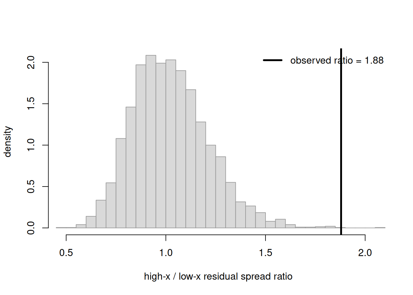
Worked example — the SAME check FAILS on a mis-specified model (recurring case)

Now we sabotage the model deliberately. We generate data whose spread grows with \(x\) (heteroscedastic: little scatter for low study hours, large scatter for high), but we still fit the constant-spread straight line and still summarize with residual SD — except this time we use a test quantity sensitive to the failure: the ratio of residual spread in the high-\(x\) half to the low-\(x\) half. A correctly specified constant-spread model produces replicates whose ratio hovers near \(1\); our mis-specified fit will look ordinary on that summary while the observed ratio sits far out, because the real data’s spread fans out and the model cannot reproduce it.

set.seed(2222)
n  <- 60
x  <- runif(n, 0, 12)
# Spread GROWS with x: this is the mis-specification the line cannot capture
y  <- 55 + 2.6 * x + rnorm(n, 0, 1.5 + 1.4 * x)

fit <- lm(y ~ x)                 # WRONG model: assumes constant spread
b   <- coef(fit); s <- summary(fit)$sigma

# Test quantity: spread ratio between high-x and low-x halves
spread_ratio <- function(xx, yy, ff) {
  rr  <- yy - (coef(ff)[1] + coef(ff)[2] * xx)
  hi  <- xx >= median(xx)
  sd(rr[hi]) / sd(rr[!hi])
}
obs_ratio <- spread_ratio(x, y, fit)

R <- 4000
rep_ratio <- numeric(R)
for (r in 1:R) {
  y_rep <- b[1] + b[2] * x + rnorm(n, 0, s)   # constant-spread replicate
  rep_ratio[r] <- spread_ratio(x, y_rep, lm(y_rep ~ x))
}

hist(rep_ratio, breaks = 30, freq = FALSE, col = "grey85", border = "grey60",
     main = "", xlab = "high-x / low-x residual spread ratio",
     ylab = "density", xlim = range(c(rep_ratio, obs_ratio)))
abline(v = obs_ratio, lwd = 3)
legend("topright", bty = "n", lwd = 3,
       legend = sprintf("observed ratio = %.2f", obs_ratio))

mean(rep_ratio >= obs_ratio)   # how often replicates are this extreme

[1] 5e-04

Histogram of the high-half to low-half residual spread ratio for replicated datasets, clustered near one between about point seven and one point four, with a solid vertical line at the observed ratio well to the right beyond almost all replicates, indicating the constant-spread model fails to reproduce the fanning-out scatter in the real data. — Figure 2: Posterior predictive check on a mis-specified model. Data were generated with spread that grows with x, but a constant-spread line was fit. The test quantity is the ratio of residual spread in the high-x half to the low-x half; replicates (which assume constant spread) cluster near one, while the observed ratio sits far in the right tail — the check flags the heteroscedasticity the model cannot capture.

The observed spread ratio sits far in the right tail, and the printed fraction of replicates that extreme is tiny. The check has flagged a real defect: the data’s scatter fans out with \(x\), but a constant-spread line cannot generate datasets that do this. Crucially, the fit of this model looked perfectly respectable — the line still ran through the middle of the points and reported tidy coefficients. Only the targeted predictive check exposed the problem. That is the lesson: a good-looking fit is not a clean bill of health.

Worked example — transfer: comparing two models for clinic walk-in counts

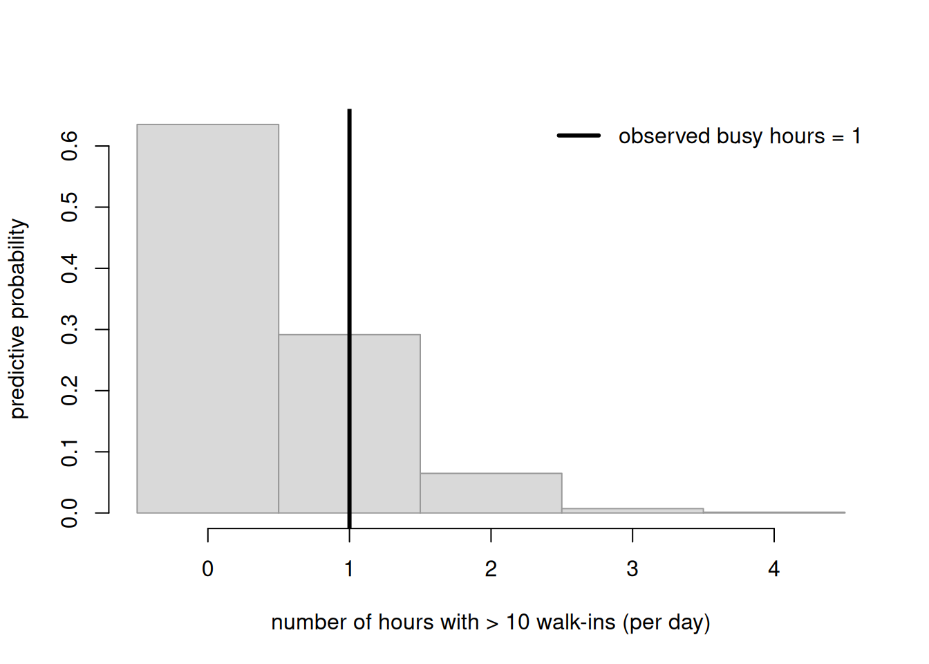
Same logic, new context, and now a comparison rather than a single check. The clinic strand from Week 7/10 counts walk-ins, and a plain Poisson model can be too rigid when busy hours are over-dispersed (more variable than Poisson allows). Suppose we have two candidates for daily walk-in counts: Model A, a single Poisson rate; Model B, a Poisson whose rate varies by time of day. A predictive check on the test quantity “number of unusually busy hours (count above a threshold) in a day” tells us which model can reproduce the bursty reality. We simulate the observed-style data with real burstiness and check Model A.

set.seed(3333)
hours <- 12
# 'Observed' day: rate varies (busy midday) -> bursty, over-dispersed
true_rate <- c(3,3,4,6,9,12,12,9,6,4,3,3)
obs_day   <- rpois(hours, true_rate)
obs_busy  <- sum(obs_day > 10)              # observed test quantity

# Model A: single Poisson rate = overall mean; replicate many days
rateA <- mean(obs_day)
R <- 5000
repA_busy <- replicate(R, sum(rpois(hours, rateA) > 10))

hist(repA_busy, breaks = seq(-0.5, max(c(repA_busy, obs_busy)) + 0.5, by = 1),
     freq = FALSE, col = "grey85", border = "grey60",
     main = "", xlab = "number of hours with > 10 walk-ins (per day)",
     ylab = "predictive probability")
abline(v = obs_busy, lwd = 3)
legend("topright", bty = "n", lwd = 3,
       legend = sprintf("observed busy hours = %d", obs_busy))

mean(repA_busy >= obs_busy)   # predictive position under Model A

[1] 0.3648

Histogram of the number of busy hours per simulated day under a single-rate Poisson model, mostly zero to two, with a solid vertical line at the observed count of busy hours further right beyond most replicates, indicating the single-rate model rarely produces days as bursty as observed. — Figure 3: Predictive check of a single-rate Poisson model (Model A) for bursty clinic walk-ins. The test quantity is the number of hours per day with more than 10 walk-ins. Replicated days from the single-rate model rarely show many busy hours, but the observed day has several, placing the observed value in the right tail — evidence that the simpler Model A under-predicts busyness and the time-varying Model B is worth its extra structure.

Under the single-rate Model A, days with several very-busy hours are rare, yet the observed day has more than the replicates typically produce — the observed value lands in the tail. This is predictive evidence that Model A is too rigid and the time-varying Model B (which can produce midday bursts) is worth its added complexity. Notice the comparison is grounded in predicting a feature we care about (burstiness), not in which model fits the training counts most tightly.

A common mistake

Believing that a model which fits the training data well is therefore a good predictive model.

This is the single most expensive misconception in applied modeling, and it sounds completely reasonable. “My polynomial passes through every point — surely it understands the data better than the boring line.” It does not. It has memorized the data, including its noise, and memorization is the opposite of prediction. The clearest tell is that adding flexibility always improves in-sample fit (more parameters can only bend closer to the points), so “better fit” carries no information about whether the extra flexibility captured real signal or just chased noise. A model can ace every in-sample number and predict new data worse than a coin-aware guess.

How to catch it: never judge a model by how well it fits the data it was trained on. Ask instead, how well would this predict data it has not seen? — and reach for an out-of-sample measure (held-out prediction, cross-validation-style scores) or, at minimum, a posterior predictive check on a summary the model was not tuned to match. And recall the maxim “all models are wrong, but some are useful”: the goal is never a perfect model, which does not exist, but a model useful for the prediction or decision at hand. Usefulness is judged out-of-sample, not by training fit.

Interpretation guidance

What a passed check certifies: that the model is capable of producing data like yours on the specific summary you tested. Nothing more. It is a consistency result, not a proof of correctness — many wrong models pass many checks, and a model that passes every summary you tried can still be wrong on one you did not think to test. A pass means “I have not found this flaw,” never “the model is true.”

What a failed check tells you and does not: a failure is a genuine, useful signal that your data is surprising under the model on that summary — it points a flashlight at a real discrepancy. It does not identify which assumption is wrong, does not prove the model is worthless (it may still be useful for other purposes), and does not prescribe the fix. The right response is to look at which summary failed, reason about what modeling change would address it, and re-check.

What a model comparison establishes and does not: a comparison says which candidate predicts a chosen target better, on the evidence so far, with uncertainty. It does not crown a “true” model, and a small score difference may be within noise — treat “A beats B” the way you treat a point estimate, as something that needs an interval before you lean on it. And remember that comparison only ranks the candidates you brought; the best model may be one neither of you wrote down.

Finally, keep the uncertainties straight (O11). Parameter uncertainty is the width of the posterior over coefficients; predictive uncertainty is the spread of future data; model uncertainty is doubt about which model form is right; model-choice uncertainty is the error in a comparison score itself. A predictive check probes the third; a model comparison engages the third and fourth. Never let a confident coefficient summary disguise the fact that the whole model might be the wrong story.

Practice (ungraded)

Use these to check your own understanding. No solutions or answer keys are posted here.

In your own words, explain the four-step posterior predictive check recipe for a regression model. Why must each replicated dataset reuse the observed \(x_i\) values?
For the study-hours model, name two test quantities other than residual SD that would be sensitive to (a) a curved relationship and (b) a single influential outlier. Say what each would look like in a failed check.
A classmate fits a 9-degree polynomial to 12 data points, reports a near-perfect in-sample fit, and concludes it is the best model. State precisely what is wrong with the reasoning and what they should measure instead.
Re-run the passing-check figure (fig-ppc-pass) but change the data-generating spread from 8 to 20. Predict, before running, whether the observed residual SD will still land in the bulk of the replicates, then check and explain.
Two models for the same data have out-of-sample predictive scores that differ by an amount smaller than the uncertainty in the difference. What should you conclude, and which model would you prefer and why?
Explain the maxim “all models are wrong, but some are useful” to a friend who has never taken statistics, using the study-hours example. What makes a wrong model still useful?

Reading guide

This week maps to Bayes Rules! Ch 10 — Evaluating regression models. Chapter 10’s three questions for any regression — is the model fair, how wrong is it, and how accurate are its predictions? — are exactly the spine of this week, even though our framing and examples are our own. Read its development of posterior predictive checks for regression as the direct generalization of the Week 6 checking idea to a whole dataset of \((x, y)\) pairs: the replicate-summarize-compare loop in our figures is the same loop the chapter describes, with our residual-spread test quantities standing in for the chapter’s summaries. Read its treatment of predictive accuracy as the formal version of our in-sample versus out-of-sample contrast, and let its cross-validation discussion ground the principle that we judge models on data they have not seen. As you read, keep our study-hours and clinic examples beside the chapter’s worked case so the structure — generate replicates from the fit, summarize, compare, then prefer the model that predicts the unseen — transfers even though the numbers differ. We adapt the chapter’s concepts in the course’s own voice and synthetic examples; the text is used under CC BY-NC-SA 4.0.

Public vs. graded

These notes and the ungraded practice above are public and for learning only. No answer keys are posted here, and nothing on this page sets graded prompts, rubric values, point values, or due dates. For anything that counts toward your grade — exit-ticket scope, quiz wording, deadlines — the LMS (Blackboard) is authoritative. Where this page and the LMS differ, the LMS governs.

Looking ahead

We have spent the term inside the Bayesian world, checking and comparing Bayesian models on their own terms. Next week — Week 12: Bayesian & classical in conversation — we step back and put Bayesian and classical summaries side by side: where they agree, where they genuinely differ, and how to read each honestly without conflating them. See Week 12 — Bayesian & classical in conversation.