Two frameworks, side by side, with the meanings kept straight
The week question
When a Bayesian credible interval and a classical confidence interval print the same two numbers, do they say the same thing — and how would you tell?
Where we are and why this matters
For eleven weeks we have built one machine: a prior \(f(\theta)\), a likelihood \(L(\theta \mid y)\), and a posterior \(f(\theta \mid y) \propto L(\theta \mid y)\, f(\theta)\). From that posterior we have read credible intervals since Weeks 4 and 5, and we have leaned on the same posterior interpretation in every week since — the parameter \(\theta\) is uncertain, the posterior describes how plausible each value is, and a 95% credible interval is a range that holds 95% of that posterior plausibility.
You did not learn this in a vacuum. Almost every other statistics course, every journal article, and every software default speaks a different dialect — the classical (frequentist) one, with its confidence intervals and p-values. Those tools answer real questions well. But they answer different questions than ours, and the single most common error in applied statistics is to read a classical result as if it were a Bayesian one. This week we put the two frameworks in the same room, without slogans and without picking a winner, so that you can read either kind of result correctly and communicate evidence responsibly — which is the professional skill that outlasts any one course.
This is a cross-cutting week: it does not introduce a new model. It sharpens how you talk about the models you already have. Keep the Bayes vs. classical cheatsheet open beside this note — it is the one-page companion to everything below.
Learning goals
By the end of this week you should be able to:
State, in your own words, what a confidence interval means and what it does not mean.
State what a p-value is — \(P(\text{data this extreme} \mid H_0)\) — and what it is not.
Explain why a credible interval and a confidence interval can agree numerically for different reasons.
Take one dataset, view it through both frameworks, and write a correct interpretation of each result.
Catch the two headline misreadings: the “95% probability the parameter is inside” slip, and “the data prove it.”
Core vocabulary
Parameter (\(\theta\)): the unknown we want to learn — for us this week, the proportion of students who bike to campus. Bayesians treat it as uncertain and give it a distribution; classical statisticians treat it as a fixed (if unknown) constant.
Credible interval: a range carrying a stated posterior probability (e.g., 95%) for \(\theta\). A direct statement about \(\theta\): “given the data and prior, there is a 95% probability \(\theta\) lies here.”
Confidence interval: a range produced by a procedure whose long-run coverage is the stated level. The 95% describes the procedure across hypothetical repeated samples, not the single interval in front of you.
Null hypothesis (\(H_0\)): a specific claim about \(\theta\) used as a reference point in classical testing (e.g., “\(p = 0.5\)”).
p-value: the probability, computed assuming \(H_0\) is true, of data at least as extreme as what you observed. A statement about the data under a hypothesis, not about the hypothesis.
Posterior probability of a hypothesis: in the Bayesian framework, \(P(H \mid y)\) — read directly off the posterior (e.g., “the posterior probability that \(p < 0.5\) is 0.91”).
The same word, two different meanings: “95%”
Both frameworks hand you an interval and a percentage. The percentage attaches to different things.
A credible interval puts the 95% on the parameter. The posterior \(f(\theta \mid y)\) is a genuine probability distribution over \(\theta\), so we are entitled to say there is a 95% probability that \(\theta\) lies in \([L, U]\). The interval is fixed once you have the data; the parameter is the uncertain object, and the probability lives on it.
A confidence interval puts the 95% on the procedure. In the classical picture \(\theta\) is a fixed constant — it is either in your interval or it is not, with no probability about it. What is random is the sampling: imagine repeating the study many times, each time computing an interval by the same recipe. A “95% confidence” procedure is one whose intervals would cover the true \(\theta\) in 95% of those hypothetical repetitions. That long-run coverage is the guarantee. It says nothing, in classical terms, about whether this particular interval contains \(\theta\).
This is why the two intervals can sit at the same coordinates and mean different things. The numbers are an output; the meaning is in which object the probability describes.
What a p-value is — and the swap that ruins it
A p-value answers a conditional question, and the direction of the conditioning is everything. It is
\[
\text{p-value} = P(\text{data at least this extreme} \mid H_0 \text{ true}).
\]
Read it left to right: assume the null is true, then ask how surprising the observed data (or something more extreme) would be under that assumption. A small p-value means “data like this would be unusual if \(H_0\) held,” which is taken as evidence against\(H_0\).
The fatal swap is to flip the conditioning and read it as
\[
P(H_0 \text{ true} \mid \text{data}),
\]
the probability that the null is true given what you saw. These are not equal, and turning one into the other is exactly the move Bayes’ rule forbids without a prior. \(P(A \mid B) \ne P(B \mid A)\) in general: the probability of a positive test given disease is not the probability of disease given a positive test — the Week 2 diagnostic example made this concrete. The p-value is the first kind of statement. The thing people want — how plausible the hypothesis is now — is the second kind, and only a Bayesian posterior delivers it.
So a Bayesian and a classical analysis can both speak about “\(p = 0.5\),” but they emit different objects: classical inference reports \(P(\text{data} \mid H_0)\); Bayesian inference can report \(P(H_0 \mid y)\) or, more usefully, the whole posterior \(f(p \mid y)\) from which any hypothesis probability follows.
Why they often nearly agree — for different reasons
If the frameworks mean different things, why do their numbers so often coincide? Because with a lot of data and a weak (diffuse) prior, the posterior is dominated by the likelihood. The prior gets swamped; the posterior centers near the maximum-likelihood estimate with a spread close to the classical standard error. So a 95% credible interval and a 95% confidence interval land in nearly the same place.
But the agreement is a coincidence of arithmetic, not of meaning. The credible interval got there by being the central 95% of a posterior distribution over \(\theta\). The confidence interval got there as the output of a procedure with 95% long-run coverage. When data are scarce, or the prior is informative and well chosen, the two can separate — and then you must know which question you actually asked. The lesson is not “they’re the same, relax.” It is “check why they match, because when they stop matching you need to know which one to trust for your question.”
Communicating evidence responsibly
The point of keeping the meanings straight is not pedantry — it is honest reporting. Three habits:
Name the object. Say “a 95% credible interval” or “a 95% confidence interval,” never a bare “95% interval.” The adjective is the meaning.
Pair the point with the interval. Report a posterior mean (or median) with its credible interval — never a point estimate alone. A single number hides the uncertainty you worked to quantify.
Use evidence verbs, not proof verbs. Data shift plausibility, support, or provide evidence for a claim. Data do not prove it. “Prove” overclaims in both frameworks.
Two analyses, side by side
The two worked examples below take a single dataset each and read it through both frameworks, so you can see exactly where the sentences diverge.
Worked example — the bike-to-campus proportion, both ways
Our recurring survey: we want \(p\), the proportion of students who bike to campus. We use a mild prior \(\text{Beta}(2,2)\) and observe \(y = 8\) bikers out of \(n = 24\) surveyed. By the Beta-Binomial update from Week 4, the posterior is
with posterior mean \((\alpha + y)/(\alpha + \beta + n) = 10/28 \approx 0.357\).
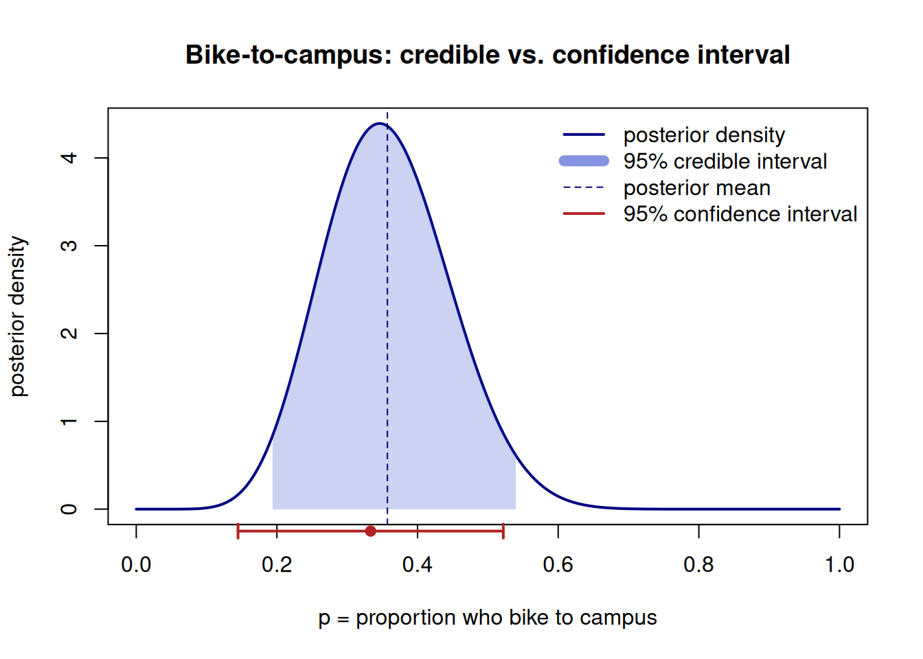
Bayesian reading. A 95% credible interval is the central 95% of \(\text{Beta}(10,18)\), computed below as roughly \([0.20, 0.53]\). Interpretation: given the prior and these data, there is a 95% probability that the bike-to-campus proportion is between about 0.20 and 0.53, with a posterior mean near 0.36. We can also read a hypothesis probability straight off the posterior — for instance, the posterior probability that \(p < 0.5\) is large (the bulk of \(\text{Beta}(10,18)\) sits below 0.5).
Classical reading. A frequentist would form a confidence interval for \(p\) from the sample proportion \(\hat p = 8/24 \approx 0.333\). A standard large-sample interval is \(\hat p \pm 1.96\sqrt{\hat p(1-\hat p)/n}\), giving roughly \(0.333 \pm 0.189 = [0.144, 0.522]\). (With only \(n = 24\) this normal approximation is rough — a reason to prefer exact methods at this sample size, but it illustrates the contrast.) Interpretation: the procedure that produced this interval covers the true \(p\) in 95% of repeated samples. It is not a 95% probability that \(p\) is in \([0.144, 0.522]\).
Notice the two intervals overlap heavily but are not identical, and the mild prior pulls the Bayesian center (\(0.357\)) slightly toward \(0.5\) relative to \(\hat p = 0.333\) — the prior’s fingerprint. Most of the difference here is interpretive, not numeric.
set.seed(1212)# Posterior Beta(10,18)a <-10; b <-18curve(dbeta(x, a, b), from =0, to =1, n =400,lwd =2, col ="navy",xlab ="p = proportion who bike to campus", ylab ="posterior density",main ="Bike-to-campus: credible vs. confidence interval")# 95% credible interval (central posterior region) -- shade itci_lo <-qbeta(0.025, a, b); ci_hi <-qbeta(0.975, a, b)xs <-seq(ci_lo, ci_hi, length.out =200)polygon(c(ci_lo, xs, ci_hi), c(0, dbeta(xs, a, b), 0),col =rgb(0.2, 0.3, 0.8, 0.25), border =NA)abline(v = a / (a + b), col ="navy", lty =2) # posterior mean# 95% classical confidence interval (normal approximation) drawn as a bracketphat <-8/24; se <-sqrt(phat * (1- phat) /24)conf_lo <- phat -1.96* se; conf_hi <- phat +1.96* seyb <--0.25# below the axissegments(conf_lo, yb, conf_hi, yb, lwd =2, col ="firebrick", xpd =TRUE)segments(c(conf_lo, conf_hi), yb -0.08, c(conf_lo, conf_hi), yb +0.08,lwd =2, col ="firebrick", xpd =TRUE)points(phat, yb, pch =19, col ="firebrick", xpd =TRUE)legend("topright", bty ="n",legend =c("posterior density", "95% credible interval","posterior mean", "95% confidence interval"),col =c("navy", rgb(0.2,0.3,0.8,0.6), "navy", "firebrick"),lwd =c(2, 8, 1, 2), lty =c(1, 1, 2, 1))cat(sprintf("Credible interval: [%.3f, %.3f]\n", ci_lo, ci_hi))
Figure 1: Posterior Beta(10,18) for the bike-to-campus proportion, with its 95% credible interval (shaded) and the classical 95% confidence interval (bracket below). The numbers nearly coincide; the meanings do not.
The takeaway is in the two printed lines: similar coordinates, different sentences attached to them.
Worked example — transfer: a clinic’s “no-wait” rate
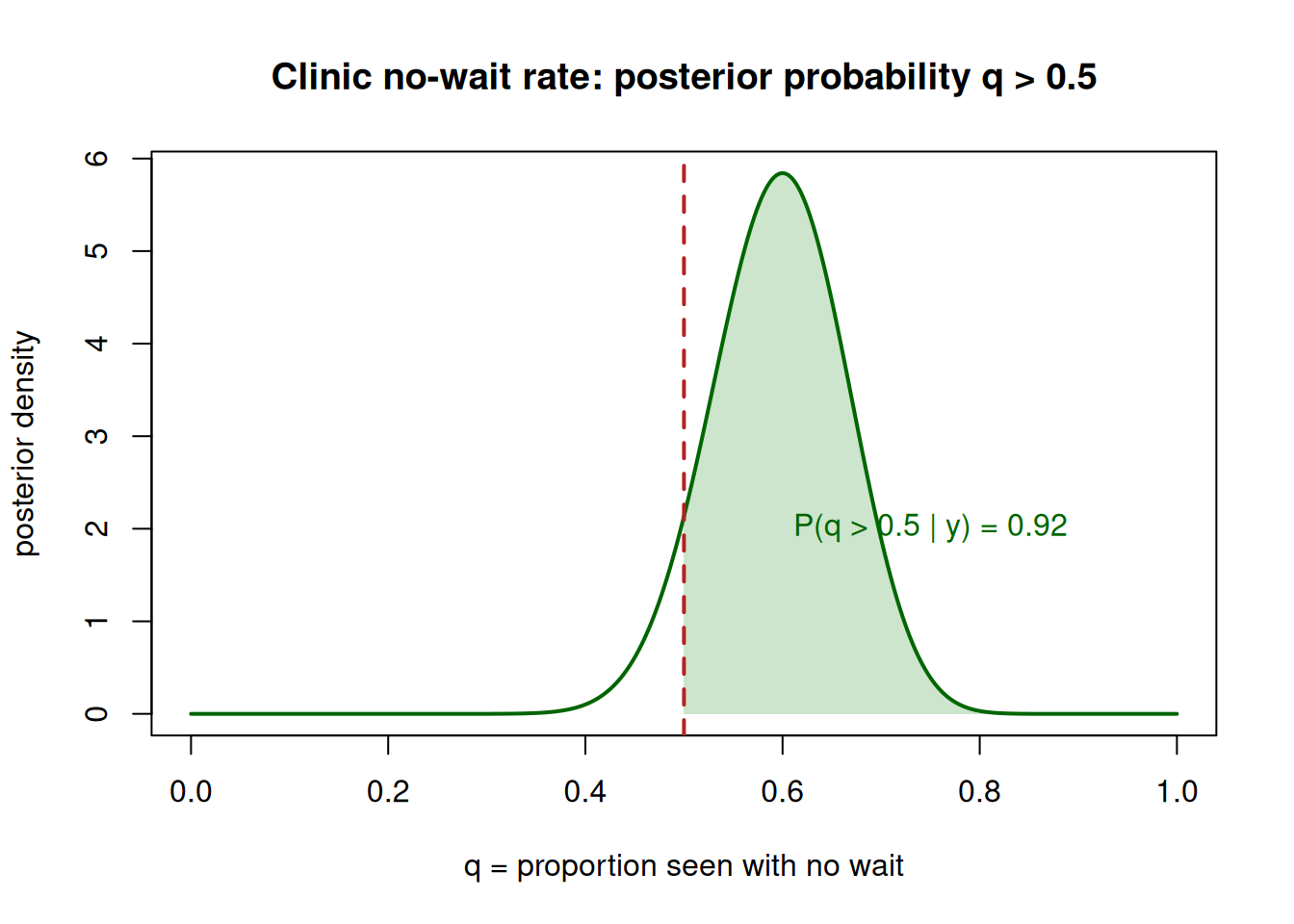
A campus clinic claims that more than half of walk-in patients are seen with no wait. To check, we treat the no-wait rate \(q\) as the parameter and survey \(y = 30\) no-wait visits out of \(n = 50\). With a flat-ish prior \(\text{Beta}(1,1)\), the Beta-Binomial update gives
Bayesian sentence. The 95% credible interval is roughly \([0.46, 0.72]\), and the posterior probability that \(q > 0.5\) is about 0.91. We can report directly: there is about a 91% posterior probability that more than half of walk-ins are seen with no wait. That sentence is the kind classical methods cannot produce.
Classical sentence. A frequentist test of \(H_0: q = 0.5\) against \(q > 0.5\) with \(\hat q = 30/50 =
0.6\) yields a one-sided p-value of roughly 0.08. The correct reading is: if the true no-wait rate were exactly 0.5, data this favorable (or more) would occur about 8% of the time. It is not “an 8% probability the claim is false.” The two analyses agree that the evidence leans toward “more than half,” but only the Bayesian one answers the question the clinic actually asked.
set.seed(50)a2 <-31; b2 <-21curve(dbeta(x, a2, b2), from =0, to =1, n =400,lwd =2, col ="darkgreen",xlab ="q = proportion seen with no wait", ylab ="posterior density",main ="Clinic no-wait rate: posterior probability q > 0.5")xs <-seq(0.5, 1, length.out =200)polygon(c(0.5, xs, 1), c(0, dbeta(xs, a2, b2), 0),col =rgb(0, 0.5, 0, 0.2), border =NA)abline(v =0.5, col ="firebrick", lwd =2, lty =2)prob_gt <-1-pbeta(0.5, a2, b2)text(0.75, 2, sprintf("P(q > 0.5 | y) = %.2f", prob_gt), col ="darkgreen")cat(sprintf("Posterior P(q > 0.5 | data) = %.3f\n", prob_gt))
Posterior P(q > 0.5 | data) = 0.920
Figure 2: Posterior Beta(31,21) for the clinic no-wait rate. The shaded region to the right of 0.5 is the posterior probability that more than half of walk-ins wait none.
A common mistake
There are two, and they are siblings.
Mistake 1 — the confidence interval as a probability statement about \(\theta\). Seeing \([0.144,
0.522]\) and writing “there’s a 95% chance \(p\) is in here” is the single most common error in applied statistics. In the classical framework \(p\) is fixed, so it is either in the interval or not — no probability applies to this interval. The 95% belongs to the procedure’s long-run coverage. Catch it by asking: what is the random thing here? If your sentence treats the interval as fixed and \(p\) as random, you are describing a credible interval and you need a posterior (and therefore a prior) to license it.
Mistake 2 — “the data prove it.” Both a small p-value and a posterior tilted toward \(H_1\) are evidence, not proof. Data shift plausibility; they do not settle the question with certainty. Catch it by replacing every “prove/disprove” with “provide evidence for/against” and seeing whether the sentence still says what you meant. If the strength of the claim collapses, the original sentence was overclaiming.
Interpretation guidance
When you report a result, the framework determines the legitimate sentence:
Credible interval (Bayesian): “Given the data and prior, there is a 95% probability \(\theta\) lies in \([L, U]\).” You may also report direct hypothesis probabilities like \(P(\theta > c \mid y)\).
Confidence interval (classical): “This interval was produced by a procedure that covers the true \(\theta\) 95% of the time in repeated sampling.” You may not attach a probability to this interval containing \(\theta\).
p-value (classical): “If \(H_0\) were true, data at least this extreme would occur with probability \(p\).” You may not read it as the probability that \(H_0\) is true.
What none of these mean: that the result is certain, that a non-significant p-value proves the null, or that overlapping intervals from two methods are the same claim. When the numbers nearly agree, report the agreement honestly and name which interval you actually computed — the reader cannot tell from the coordinates alone.
Practice (ungraded)
Use these to check your understanding. No answers are posted here.
A study reports a 95% confidence interval for a proportion as \([0.41, 0.59]\). Write one sentence that interprets it correctly, and one common sentence that interprets it incorrectly, and say what makes the second one wrong.
For the bike survey posterior \(\text{Beta}(10,18)\), the posterior probability that \(p < 0.5\) is large. Explain why a p-value from a classical test of \(H_0: p = 0.5\) is not the complement of that probability.
Two analysts study the same large dataset with a weak prior; their credible and confidence intervals nearly coincide. A third analyst concludes “so the frameworks are equivalent.” Where does that conclusion go too far?
Rewrite this sentence responsibly: “The experiment proved that the new study method raises exam scores (\(p = 0.03\)).”
Re-run the fig-bike-two-intervals chunk with \(\text{Beta}(2,2)\) and a larger sample carrying the same proportion (e.g., 32 of 96). Do the credible and confidence intervals move closer together? Explain why in terms of the prior being swamped.
Reading guide
This week is cross-cutting, so we lean on two Bayes Rules! chapters for the conceptual contrast rather than a single new model.
Ch 1 (The big Bayesian picture): read for the foundational distinction between probability as long-run frequency (classical) and probability as plausibility about \(\theta\) (Bayesian). That one distinction is the root of every difference in this note — it is why “95%” attaches to a procedure in one framework and to the parameter in the other. Map their framing onto our “## The same word, two different meanings” section.
Ch 8 (Posterior inference & summaries): revisit the credible-interval definition and how to read a posterior summary. Use it to anchor the Bayesian sentences in both worked examples; the chapter gives the posterior-probability reading we contrast with the confidence interval here.
We adapt these chapters’ ideas in the course’s own voice and examples; we do not reproduce their text, figures, or datasets. Bayes Rules! is CC BY-NC-SA 4.0.
Public vs. graded
This is a public, ungraded note. The quizzes, homework, and exams that carry your grade live in the LMS (Blackboard), which is authoritative for all graded prompts, weights, due dates, and keys — no answer keys are posted here. The Practice prompts above are for self-study only.
Looking ahead
Next week we keep the parameter uncertain but let it vary across groups: Week 13 — Hierarchical models, where exam scores across several sections share strength through partial pooling, so that small or noisy groups borrow information from the rest.