Week 10 — Bayesian regression II

More predictors, binary outcomes, and prediction that carries its uncertainty

Mathematical goal

Week 9 fit a single straight line to a continuous outcome. This week the goal is to write down — and read off — two extensions of that model that are not optional decorations but the workhorses of applied Bayesian modeling. First, we extend the linear predictor from one slope to several: a coefficient for each of several predictors, each interpreted holding the others fixed. Second, we change the outcome type: when the response is binary (yes/no, success/failure) a straight line through it is nonsensical, so we model the log-odds of success as linear in the predictors — logistic regression. We will state both models precisely, derive how a single logistic coefficient becomes an odds ratio on the multiplicative scale, and insist throughout that any prediction we produce comes with a posterior — a distribution, not a number.

The mathematical objects do not change from earlier weeks. We still have a prior \(f(\theta)\) over parameters \(\theta\), a likelihood \(L(\theta \mid y)\) from the data model, and a posterior \(f(\theta \mid y) \propto L(\theta \mid y)\, f(\theta)\). What changes is the shape of \(\theta\) (now a vector of coefficients) and the form of the data model (Bernoulli through a link, rather than Normal).

Notation

This week introduces vector-valued parameters and a link function. The notation below extends the fixed course conventions; nothing here overrides them.

Symbol	Reads as	Note
\(y_i\)	the outcome for observation \(i\)	binary (\(0/1\)) in logistic regression
\(x_{i1}, x_{i2}, \dots, x_{ik}\)	the \(k\) predictor values for observation \(i\)	one column per predictor
\(\beta_0\)	the intercept coefficient	a parameter, so it has a prior
\(\beta_1, \dots, \beta_k\)	the slope coefficients	one per predictor; each a parameter
\(\pi_i\)	\(P(y_i = 1)\), the success probability for observation \(i\)	lives in \((0,1)\)
\(\eta_i\)	the linear predictor \(\beta_0 + \beta_1 x_{i1} + \cdots\)	lives on the whole real line
\(\theta\)	the full parameter vector \((\beta_0, \beta_1, \dots, \beta_k)\)	(plus the noise sd in the Normal case)
\(\operatorname{odds}(\pi)\)	\(\pi / (1-\pi)\)	the odds of success
\(\operatorname{logit}(\pi)\)	\(\log\!\big(\pi/(1-\pi)\big)\)	the log-odds; the logistic link

The prior is \(f(\theta)\), the likelihood \(L(\theta \mid y)\) is a function of \(\theta\) (not a distribution over it), and the posterior is \(f(\theta \mid y)\). The symbol \(\propto\) continues to mean “equal up to a constant that does not depend on \(\theta\)”; what it drops is the marginal \(f(y)\).

Conceptual setup

Recall the Week 9 setup: \(y_i = \beta_0 + \beta_1 x_i + \varepsilon_i\) with \(\varepsilon_i \sim N(0,\sigma^2)\), priors on \(\beta_0,\beta_1,\sigma\), and a posterior over the coefficients. Two assumptions in that line are worth naming because this week relaxes or replaces them.

The first assumption is that one predictor is enough. Almost never true. If exam score depends on both study hours and prior GPA, a model with only study hours forces the GPA effect to hide inside the study-hours slope, biasing it. The fix is honest: give each predictor its own coefficient. The linear predictor becomes a sum, and we assume (to start) that effects are additive — each predictor contributes its slope times its value, and the coefficients add. We also assume each slope is a partial effect: the change in the expected outcome for a one-unit change in that predictor with the other predictors held fixed. That conditioning phrase is the whole interpretive content of multiple regression; drop it and you will misread every coefficient.

The second assumption is that the outcome is continuous and a straight line through it is meaningful. For a binary outcome \(y_i \in \{0,1\}\) this fails. A line \(\beta_0 + \beta_1 x_i\) ranges over the whole real line, but a probability must sit in \((0,1)\); a linear model will happily predict \(1.3\) or \(-0.2\). The remedy is to keep the linear predictor on the real line but link it to the probability through a squashing function. We model the log-odds as linear: \(\operatorname{logit}(\pi_i) = \eta_i\), which means \(\pi_i = 1/(1+e^{-\eta_i})\) always lands in \((0,1)\). The data model is then Bernoulli: \(y_i \mid \pi_i \sim \text{Bernoulli}(\pi_i)\).

Crucially, the Bayesian object is still a posterior over coefficients. Because each draw of \((\beta_0,\beta_1,\dots)\) from the posterior implies a whole fitted curve, the Bayesian view of a logistic fit is not one S-curve but a posterior bundle of S-curves — and any predicted probability inherits that spread. Hold onto this: prediction is a distribution.

The multiple-predictor model statement

With \(k\) predictors and a continuous outcome, the model is

\[ y_i = \beta_0 + \beta_1 x_{i1} + \beta_2 x_{i2} + \cdots + \beta_k x_{ik} + \varepsilon_i, \qquad \varepsilon_i \sim N(0, \sigma^2), \]

with independent priors on \(\beta_0, \beta_1, \dots, \beta_k\) and on \(\sigma\). The posterior \(f(\beta_0,\dots,\beta_k,\sigma \mid y) \propto L(\beta_0,\dots,\sigma \mid y)\, f(\beta_0,\dots,\sigma)\) is now a joint distribution over all the coefficients at once. We summarize it the same way as before, one coefficient at a time: report each coefficient’s posterior mean (or median) together with a credible interval — never a point alone. The interpretation of \(\beta_j\) is the partial effect: the expected change in \(y\) per one-unit change in \(x_j\), the other predictors held fixed.

The logistic model statement

For a binary outcome the model is

\[ y_i \mid \pi_i \sim \text{Bernoulli}(\pi_i), \qquad \operatorname{logit}(\pi_i) = \log\!\frac{\pi_i}{1-\pi_i} = \beta_0 + \beta_1 x_{i1} + \cdots + \beta_k x_{ik}. \]

Inverting the link gives the success probability directly:

\[ \pi_i = \frac{1}{1 + e^{-(\beta_0 + \beta_1 x_{i1} + \cdots + \beta_k x_{ik})}}. \]

Priors go on \(\beta_0,\dots,\beta_k\) as usual, and the posterior \(f(\beta_0,\dots,\beta_k \mid y) \propto L(\beta_0,\dots,\beta_k \mid y)\, f(\beta_0,\dots,\beta_k)\) is a joint distribution over the coefficients. There is no separate noise sd here: the Bernoulli variance \(\pi_i(1-\pi_i)\) is already pinned down by \(\pi_i\).

From a logistic coefficient to an odds ratio

The reason logistic coefficients are interpreted on the odds scale is a one-line piece of algebra, and it is the most useful derivation of the week. Take a single predictor \(x\) and compare the odds at \(x\) to the odds at \(x+1\) (the other predictors, if any, held fixed). By the model,

\[ \operatorname{odds}(\pi \mid x) = \frac{\pi}{1-\pi} = e^{\,\beta_0 + \beta_1 x}. \]

Step the predictor up by one unit:

\[ \operatorname{odds}(\pi \mid x+1) = e^{\,\beta_0 + \beta_1 (x+1)} = e^{\,\beta_0 + \beta_1 x}\, e^{\beta_1}. \]

Divide the second by the first and the intercept and the \(x\) term cancel:

\[ \frac{\operatorname{odds}(\pi \mid x+1)}{\operatorname{odds}(\pi \mid x)} = e^{\beta_1}. \]

So \(e^{\beta_1}\) is the odds ratio for a one-unit increase in \(x\): a multiplicative factor on the odds, not an additive change in the probability. A coefficient of \(\beta_1 = 0\) gives odds ratio \(e^0 = 1\) (no effect); \(\beta_1 > 0\) gives a ratio above \(1\) (odds increase); \(\beta_1 < 0\) gives a ratio below \(1\) (odds decrease). Because \(\beta_1\) is a parameter with a posterior, the odds ratio \(e^{\beta_1}\) is itself a posterior quantity: transform each posterior draw of \(\beta_1\) through \(\exp(\cdot)\) and you get a posterior — and hence a credible interval — for the odds ratio.

Worked example — symbolic: a coefficient becomes an odds ratio

Take a one-predictor logistic model for whether a student passes a checkpoint (\(y_i = 1\) for pass) as a function of hours of focused review \(x_i\):

\[ y_i \mid \pi_i \sim \text{Bernoulli}(\pi_i), \qquad \operatorname{logit}(\pi_i) = \beta_0 + \beta_1 x_i. \]

Suppose the posterior for the slope is centered at \(\beta_1 = 0.40\) with a \(95\%\) credible interval \([0.15,\ 0.66]\). On the odds scale the point summary is

\[ e^{\beta_1} = e^{0.40} \approx 1.49, \]

and transforming the interval endpoints gives an odds-ratio credible interval

\[ \big[e^{0.15},\ e^{0.66}\big] \approx [1.16,\ 1.93]. \]

Reading: each additional hour of focused review multiplies the odds of passing by about \(1.49\) — a \(49\%\) increase in the odds — and we are about \(95\%\) posterior-confident the multiplier lies between roughly \(1.16\) and \(1.93\). The whole interval sits above \(1\), so the data, filtered through the prior, push toward a positive association. Note what we did not say: we did not say the probability of passing rises by a fixed amount per hour. It does not — the probability change depends on where you start on the S-curve, which is exactly the point of the next example.

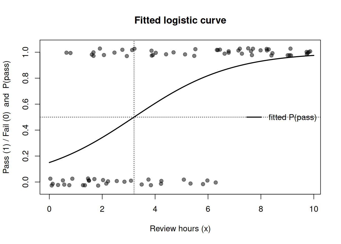
Worked example — numeric instance you can re-run: a fitted logistic curve

The chunk below builds a small synthetic dataset (pass/fail versus review hours), fits a logistic model with glm, draws the fitted S-curve, and prints the slope and its implied odds ratio. The glm fit is a maximum-likelihood point summary; read the figure caption for how the Bayesian posterior-over- curves view sits on top of it. All randomness is seeded, so you get the same numbers every time.

set.seed(1010)
n <- 80
hours <- runif(n, 0, 10)                       # synthetic review hours
eta   <- -2.0 + 0.55 * hours                   # true log-odds (linear predictor)
pi    <- 1 / (1 + exp(-eta))                   # true success probabilities
y     <- rbinom(n, size = 1, prob = pi)        # observed pass/fail

fit <- glm(y ~ hours, family = binomial)       # logistic regression by ML
b   <- coef(fit)                               # intercept and slope estimates

# scatter with light vertical jitter so 0/1 points are visible
plot(hours, y + runif(n, -0.03, 0.03),
     pch = 19, col = rgb(0, 0, 0, 0.5),
     xlab = "Review hours (x)", ylab = "Pass (1) / Fail (0)  and  P(pass)",
     ylim = c(-0.05, 1.05), main = "Fitted logistic curve")

# overlay the fitted probability curve
xx <- seq(0, 10, length.out = 200)
pp <- 1 / (1 + exp(-(b[1] + b[2] * xx)))
lines(xx, pp, lwd = 2)
abline(h = 0.5, lty = 3); abline(v = -b[1] / b[2], lty = 3)  # where P(pass) = 0.5
legend("right", legend = "fitted P(pass)", lwd = 2, bty = "n")

Scatter of binary outcomes at heights zero and one across review hours from zero to ten, overlaid with a rising S-shaped logistic curve climbing from near zero probability on the left to near one on the right, crossing one-half around four to five hours. — Figure 1: Synthetic pass/fail data (jittered points at y = 0 and y = 1) with the fitted logistic curve giving P(pass) as a function of review hours. The single solid curve is the maximum-likelihood (glm) fit; in the Bayesian view each posterior draw of the coefficients yields one such curve, so the honest picture is a *bundle* of curves whose vertical spread at any x is the posterior uncertainty in the predicted probability.

slope    <- coef(fit)["hours"]
odds_rat <- exp(slope)                          # odds ratio per extra hour
round(c(slope = unname(slope), odds_ratio = unname(odds_rat)), 3)

     slope odds_ratio 
     0.541      1.718

The printed slope is the estimated log-odds change per extra hour; exp(slope) is the estimated odds ratio. Because we generated the data with a true slope of \(0.55\), the estimate should land near there, and the odds ratio near \(e^{0.55}\approx 1.73\). To make the Bayesian uncertainty concrete without extra packages, you can also see the S-curve steepest near \(P=0.5\) and flat at the extremes — which is why a fixed change in \(x\) moves the probability a lot in the middle and barely at all near \(0\) or \(1\).

A transfer case — counts go to Poisson regression

The same link-the-linear-predictor recipe handles count outcomes. The clinic wait-time strand from Week 7 is the natural carrier: suppose instead of wait times we count the number of walk-ins per hour, \(y_i \in \{0,1,2,\dots\}\), as a function of, say, the hour of day. A count cannot be Normal (it is non-negative and discrete) and its mean must stay positive, so we use a log link:

\[ y_i \mid \lambda_i \sim \text{Poisson}(\lambda_i), \qquad \log(\lambda_i) = \beta_0 + \beta_1 x_{i1} + \cdots. \]

Here \(e^{\beta_1}\) is a rate ratio: a one-unit increase in \(x_1\) multiplies the expected count by \(e^{\beta_1}\) — exactly parallel to the odds-ratio derivation above, with “odds” replaced by “rate.” The Bayesian machinery is identical: priors on the coefficients, a posterior over them, point-plus-interval summaries, and prediction reported as a distribution. (Bayes Rules! Ch 12 develops this case in full; we only flag it here so the pattern — pick a data model, link the linear predictor, keep the posterior — is visible as one idea, not three.)

A convention warning

Two cautions, both about reading coefficients honestly; treat them as the non-negotiable conventions of the week.

The first convention concerns log-odds versus probability. A logistic coefficient \(\beta_1\) lives on the log-odds scale; \(e^{\beta_1}\) is a multiplicative effect on the odds; neither is a change in probability. The probability effect of a one-unit change in \(x\) is not constant — it depends on where you sit on the S-curve, large near \(\pi = 0.5\) and tiny near \(0\) or \(1\). So “the coefficient is \(0.40\), so probability rises \(0.40\)” is simply wrong, and “the odds ratio is \(1.49\), so probability rises \(49\%\)” is also wrong (odds, not probability). Caution: state which scale you are on every single time.

The second convention is the one this course repeats all term: a prediction must carry its uncertainty, and you must say which uncertainty. A predicted probability or count from a Bayesian model is a posterior distribution, summarized by a point estimate paired with a credible interval — never a bare number, and never a confidence interval (a credible interval is a direct posterior probability statement about the quantity; a confidence interval is a frequentist statement about the procedure across hypothetical repetitions — do not conflate them). And distinguish the two kinds of predictive uncertainty (SLO O11): uncertainty in the fitted curve (our posterior ignorance about the coefficients, which shrinks as data grow) versus uncertainty in a new individual outcome (the irreducible randomness of a single Bernoulli or Poisson draw, which does not vanish with more data). A posterior-predictive interval for one new student folds in both; a credible interval for the success probability folds in only the first.

Practice (ungraded)

Use these to check your understanding. No answer keys appear here.

Write the one-predictor logistic model for whether a survey respondent bikes to campus as a function of distance-from-campus (km). Identify \(\pi_i\), \(\eta_i\), and which quantity is the parameter.
A logistic slope has posterior mean \(-0.30\). Compute the implied odds ratio and translate it into one plain-English sentence about the odds. Is the association positive or negative?
Explain, in two sentences, why the probability change for a one-unit increase in a predictor is larger near \(\pi = 0.5\) than near \(\pi = 0.95\). A sketch of the S-curve may help.
For the multiple-predictor Normal model, state in words what “the posterior mean of \(\beta_2\) is \(1.7\) with credible interval \([0.4, 3.0]\)” means, including the held-fixed clause.
A classmate reports a single predicted pass probability of \(0.62\) with no interval. Name what is missing and which two kinds of uncertainty a full posterior-predictive statement would include.
Re-run the figure chunk with the true slope changed from \(0.55\) to \(0.20\). Predict, before running, whether the fitted S-curve gets steeper or flatter, then check.

Formula-verification status

These formulas are prepared as evidence but NOT yet human/source verified (verified: false); see the notation ledger. The course math gate is blocked pending sign-off. Specifically, the multiple-predictor model statement, the logistic link and its inverse, the odds-ratio derivation (\(e^{\beta_1}\)), and the Poisson log-link rate-ratio claim are staged as candidate results for review, not as confirmed course truth. Do not treat any displayed identity here as final until the verification sign-off is recorded in the notation ledger and the gate is cleared.

Reading guide

Bayes Rules! Ch 11 (extending regression to several predictors) supports the multiple-predictor section above.
Bayes Rules! Ch 13 (logistic regression) supports the binary-outcome / log-odds section — read it to see the link function developed at length.
Bayes Rules! Ch 12 (Poisson regression) supports the count-outcome transfer case we sketch. Use these chapters as enrichment for the models introduced here; the page already carries the core ideas.

Public vs. graded

This page is a public, ungraded study note. Graded quiz prompts, their wording, point values, rubrics, keys, and due dates are not here: the LMS (Blackboard) is authoritative for all graded specifics, and no answer keys are posted here. The practice prompts above are for self-check only.

Looking ahead

Next week — Week 11: Model checking & comparison — we stop assuming our regression is right and start interrogating it: posterior predictive checks, comparing competing models, and deciding which one to trust. See Week 11 — Model checking & comparison.