Week 7 — Simulation-first computation

Grid approximation, posterior draws, and a reproducible Quarto workflow

The idea

Up to now we have leaned on conjugacy: a Beta prior met a Binomial likelihood and the posterior came out as another Beta, with parameters we could update by hand. That is a gift, not a guarantee. Most realistic models are not conjugate — the posterior \(f(\theta \mid y)\) exists, but no clean formula falls out. The central concept of this week is that we do not actually need a formula. If we can evaluate the unnormalized posterior at many values of \(\theta\), or sample from the posterior, we can answer every question we care about — posterior mean, credible interval, predictive checks — by computing on those numbers instead of solving an integral.

That reframing is the whole idea: a posterior is something you can compute with, not just something you write down. We will meet two computational paths. Grid approximation chops the parameter space into a fine grid, evaluates prior \(\times\) likelihood at each grid point, normalizes, and then treats the result as a discrete approximation we can sample from. Markov chain Monte Carlo (MCMC) takes a cleverer route that scales to many parameters, and we introduce it conceptually — what it does and how to ask “did it converge?” — without the theory. Both produce the same kind of output we will reuse all term: a big pile of posterior draws of \(\theta\).

Because the right answer for our recurring bike-proportion problem is already known (it is conjugate, so we have the exact Beta), this week is the perfect place to learn the machinery: we can check the approximation against the truth. That is the discipline of simulation-first computation — always compute the thing you can verify before you trust the thing you cannot.

Where we are and why this matters

In Weeks 3–4 we built the Beta-Binomial model for an unknown proportion \(p\): the proportion of students who bike to campus. With a mild prior \(\text{Beta}(2,2)\) and a synthetic survey of 8 bikers out of 24 surveyed, the conjugate update gave a posterior \(\text{Beta}(10,18)\) with posterior mean \(10/28 \approx 0.357\). In Weeks 5–6 we stress-tested that posterior with prior sensitivity and built posterior-predictive reasoning — asking what future survey counts the model expects.

This week takes those exact same ideas and computes them rather than solving them. We will grid-approximate the \(\text{Beta}(10,18)\) posterior and confirm the grid recovers the mean we already know. We will draw thousands of samples and read the posterior off the histogram. The payoff is general: once you can approximate a posterior you can write down, you can approximate one you cannot — which is exactly what real models demand. This is the computation week of the course, and the habits you build here (seeds, code-with-interpretation, rendered reports) carry into every later week, especially regression (Weeks 9–11) and hierarchical models (Week 13), where conjugacy is gone.

Learning goals

By the end of this week you should be able to:

Explain why we approximate a posterior at all, and when conjugacy is not available.
Build a grid approximation: evaluate prior \(\times\) likelihood on a grid, normalize, and sample.
Read posterior summaries (mean, credible interval) off a set of posterior draws.
Describe, in plain language, what MCMC does and what “did it converge?” is checking.
Assemble a reproducible Quarto report: seeded code, output, and interpretation together, with session info, rendered to HTML.
Recognize and fix the common runtime failures (R not found, unseeded simulation, a chunk error).

These goals serve course outcomes O5 (compute and summarize a posterior) and O13 (produce a reproducible computational workflow).

Setup

First, make sure your local toolchain is alive: R computes, VS Code edits, and Quarto renders. If you have not done this, work through the setup page before going further — a render that cannot find R will stop you cold, and we would rather discover that now than during the lab.

Then, open a fresh .qmd and confirm a trivial chunk runs. Everything this week uses base R only — no add-on packages — so if R is discoverable, you have everything you need. We will rely on seq, dbeta, sample, mean, quantile, hist, curve, and lines. Keep a habit from the very first chunk: set a seed. Any line of code that draws random numbers must be preceded (in the same reproducible document) by set.seed(...), so that “run it again” gives the same figure.

Grid approximation, step by step

A grid approximation turns a continuous posterior into a fine discrete one. The recipe is short and every step is something base R does in one line.

Lay down a grid. Choose many evenly spaced candidate values of \(\theta\) across its range. For a proportion, \(\theta \in [0,1]\), so a grid like seq(0, 1, length.out = 1001) works.
Evaluate prior \(\times\) likelihood at each grid point. The unnormalized posterior is \(L(\theta \mid y)\, f(\theta)\). For the bike problem, \(f(\theta)\) is the \(\text{Beta}(2,2)\) density and \(L(\theta \mid y)\) is the Binomial likelihood for 8 successes in 24 trials. Multiply them.
Normalize. Divide each value by the sum of all of them, so the grid values add to 1. This is the discrete stand-in for dividing by the evidence \(f(y)\) — the constant that \(\propto\) usually drops in \(f(\theta \mid y) \propto L(\theta \mid y)\, f(\theta)\). On a grid we get to compute it.
Sample. Draw grid values with replacement, with probabilities equal to the normalized weights. The result is a set of posterior draws you can summarize like any data: mean, quantile, hist.

The finer the grid and the more draws, the closer this gets to the exact posterior. The beauty is that nothing in steps 1–4 used the fact that the bike model is conjugate. The same four steps work for a posterior with no closed form — you just swap in whatever prior and likelihood you have.

# Bike proportion: prior Beta(2,2), data 8 successes in 24 trials -> exact Beta(10,18)
theta <- seq(0, 1, length.out = 1001)        # the grid
prior <- dbeta(theta, 2, 2)                    # Beta(2,2) prior density
like  <- dbinom(8, size = 24, prob = theta)    # Binomial likelihood, y=8, n=24
unnorm <- like * prior                          # prior x likelihood (unnormalized posterior)
post_grid <- unnorm / sum(unnorm)               # normalize so weights sum to 1

# Plot the EXACT posterior as a density, overlay the grid as a comparable density
exact <- dbeta(theta, 10, 18)
plot(theta, exact, type = "l", lwd = 2,
     xlab = expression(theta ~ "(proportion who bike)"), ylab = "posterior density",
     main = "Grid approximation vs exact Beta(10,18)")
# scale grid weights back to density units (divide by grid spacing) for an honest overlay
grid_density <- post_grid / (theta[2] - theta[1])
points(theta[seq(1, 1001, by = 20)], grid_density[seq(1, 1001, by = 20)],
       pch = 1, cex = 0.7)
abline(v = 10/28, lty = 2)
legend("topright", legend = c("exact Beta(10,18)", "grid approximation", "posterior mean"),
       lty = c(1, NA, 2), pch = c(NA, 1, NA), lwd = c(2, NA, 1), bty = "n")

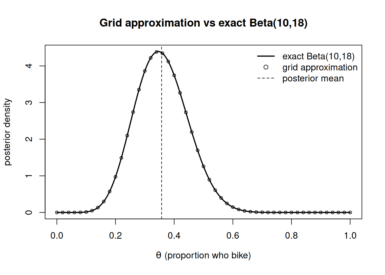
A density curve for the exact Beta(10,18) posterior rising from near zero, peaking just below 0.36, and falling toward 0.7, with small open circles from the grid approximation sitting almost exactly on the curve. A vertical dashed line marks the posterior mean at about 0.357. — Figure 1: Grid-approximated posterior for the bike proportion (points) against the exact Beta(10,18) posterior (curve). The grid recovers the closed-form shape; both peak near 0.36.

The grid points sit essentially on top of the exact curve. That visual agreement is the verification: when the truth is known, the approximation reproduces it, which licenses us to trust the method when the truth is not known.

Posterior draws are the working currency

Once we have sampled, we no longer talk to a formula — we talk to a vector of draws. Every summary is now an ordinary computation on that vector. The posterior mean is mean(draws). A 95% credible interval is quantile(draws, c(0.025, 0.975)) — and notice we say credible interval, the probability statement about \(\theta\) given the data, never confidence interval. The posterior median is median(draws). We always report a point estimate with an interval, never a point alone.

set.seed(2026)
theta <- seq(0, 1, length.out = 1001)
prior <- dbeta(theta, 2, 2)
like  <- dbinom(8, size = 24, prob = theta)
post_grid <- (like * prior) / sum(like * prior)

draws <- sample(theta, size = 20000, replace = TRUE, prob = post_grid)
sim_mean <- mean(draws)
ci <- quantile(draws, c(0.025, 0.975))

hist(draws, breaks = 40, freq = FALSE, col = "grey90", border = "white",
     xlab = expression(theta), main = "20,000 posterior draws (grid-sampled)")
abline(v = sim_mean, lwd = 2)
abline(v = ci, lty = 2)
legend("topright",
       legend = c(sprintf("simulated mean = %.3f", sim_mean),
                  sprintf("95%% CI = [%.3f, %.3f]", ci[1], ci[2])),
       lty = c(1, 2), lwd = c(2, 1), bty = "n")

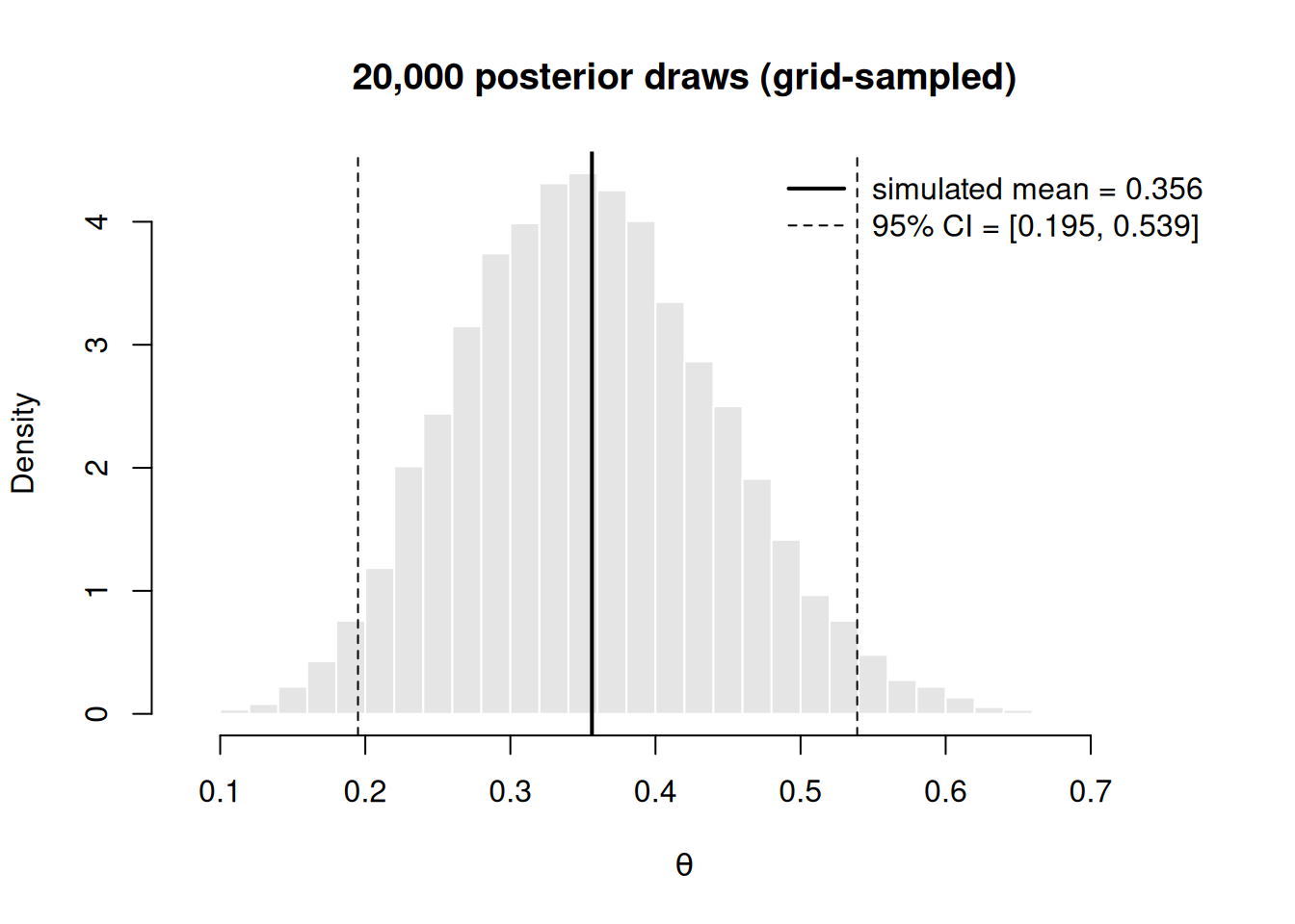
A roughly bell-shaped histogram of posterior draws centered near 0.36, ranging from about 0.2 to 0.55. A solid vertical line marks the simulated mean near 0.357; two dashed vertical lines mark the lower and upper bounds of the 95 percent credible interval at roughly 0.20 and 0.53. — Figure 2: Histogram of 20,000 posterior draws sampled from the grid approximation of the bike-proportion posterior, with the simulated mean (solid) and a 95 percent credible interval (dashed). The simulated mean lands at about 0.357, matching the closed-form value.

The simulated mean prints at about 0.357 — the same \(10/28\) we computed by hand in Week 3. That match is not luck; it is the point. When you cannot check against a formula, this same code still produces a defensible mean and interval, and you trust it because you watched it pass the check here.

MCMC, conceptually

Grid approximation is wonderful for one or two parameters and miserable for many: a grid over ten parameters has astronomically many cells. MCMC is the workhorse that scales. The concept, stripped of theory: instead of evaluating the posterior everywhere, MCMC takes a guided random walk through the parameter space that is designed to spend time in each region in proportion to its posterior probability. The sequence of places it visits — the chain — becomes your set of posterior draws, and you summarize it exactly as before: mean, quantile, hist.

You do not need the algorithm to use it responsibly, but you do need one habit: ask “did it converge?” A chain has to “forget” where it started and settle into sampling the real posterior. Two cheap diagnostics, which the course packages compute for you:

Trace plots — a plot of the chain’s value over its iterations. A converged chain looks like a fuzzy, stationary horizontal band (“a hairy caterpillar”); a chain that is wandering, trending, or stuck has not converged.
Running several chains from different starts and checking they overlap. If independent chains land on the same distribution, that is evidence they found it. (The numeric summary of this is called R-hat; you want it near 1.)

We introduce MCMC now so the idea is in place; the dedicated tooling appears later in the course. The mental model to keep: MCMC gives you posterior draws, and draws are something you already know how to summarize. Below is illustrative code in the style the course packages use — it is shown, not run.

# illustrative — runs with the course packages (rstanarm), not executed here
library(rstanarm)
fit <- stan_glm(bikes ~ 1, data = survey, family = binomial,
                prior_intercept = normal(0, 1), seed = 2026,
                chains = 4, iter = 2000)
plot(fit, "trace")        # eyeball convergence: hairy caterpillars
summary(fit)              # look for Rhat near 1
posterior <- as.data.frame(fit)   # the draws — summarize like any vector

Reproducible workflow

A result you cannot regenerate is a rumor. The deliverable of this week’s habits is a single .qmd file that holds code, output, and interpretation together and renders to a clean report. The organizing principles:

One file, one story. The .qmd is the source of truth. Prose, code chunks, and the figures they produce live in the same document, in reading order. A reader (and future you) sees the claim and the code that backs it side by side.
Seed every simulation. Put set.seed(...) in any chunk that draws random numbers, so that render reproduces the exact figure. An unseeded simulation gives a different answer each render — fine for nothing you want to defend.
Interpret next to the number. After each figure or summary, write one or two sentences saying what it means. Code that is never interpreted is not yet a result.
Save a session record. End the report with a chunk that prints sessionInfo() (R version and loaded packages). When a future render breaks, the session record is your first clue.
Render to share. Run quarto render report.qmd to produce the HTML (or PDF). You hand in the rendered report and the .qmd so a grader can re-run it.

# A session record at the foot of every reproducible report
sessionInfo()

R version 4.6.0 (2026-04-24)
Platform: x86_64-pc-linux-gnu
Running under: Ubuntu 24.04.4 LTS

Matrix products: default
BLAS:   /usr/lib/x86_64-linux-gnu/openblas-pthread/libblas.so.3 
LAPACK: /usr/lib/x86_64-linux-gnu/openblas-pthread/libopenblasp-r0.3.26.so;  LAPACK version 3.12.0

locale:
 [1] LC_CTYPE=C.UTF-8       LC_NUMERIC=C           LC_TIME=C.UTF-8       
 [4] LC_COLLATE=C.UTF-8     LC_MONETARY=C.UTF-8    LC_MESSAGES=C.UTF-8   
 [7] LC_PAPER=C.UTF-8       LC_NAME=C              LC_ADDRESS=C          
[10] LC_TELEPHONE=C         LC_MEASUREMENT=C.UTF-8 LC_IDENTIFICATION=C   

time zone: UTC
tzcode source: system (glibc)

attached base packages:
[1] stats     graphics  grDevices utils     datasets  methods   base     

loaded via a namespace (and not attached):
 [1] compiler_4.6.0  fastmap_1.2.0   cli_3.6.6       tools_4.6.0    
 [5] htmltools_0.5.9 yaml_2.3.12     rmarkdown_2.31  knitr_1.51     
 [9] jsonlite_2.0.0  xfun_0.58       digest_0.6.39   rlang_1.2.0    
[13] evaluate_1.0.5

That single rendered .qmd — seeded chunks, figures, interpretation, session info — is the artifact the rest of the course expects you to be able to produce on demand.

When it breaks

Computation fails in a few predictable ways. Recognizing the symptom is most of the fix.

“Quarto can’t find R” / the render errors before any chunk runs. Quarto must locate R to execute {r} chunks. If the render fails complaining it cannot find R, R is off your PATH. Fix: put R’s bin on PATH, set the QUARTO_R environment variable, or render from a shell whose PATH already includes R’s bin. (This is exactly the runner’s situation in this course: R 4.6.0 is installed but off PATH, so the build prepends R’s bin before quarto render.) See the setup page.
A figure changes every time you render — an unseeded simulation. Symptom: your mean and interval drift between renders. Troubleshoot by searching for any sample, rbeta, rnorm not preceded by set.seed(...) in the same chunk or document. Add the seed; the figure freezes.
A chunk error halts the whole render. One broken chunk stops the document — nothing after it builds. Fix by isolating: run the failing chunk interactively in the R console, read the error message (a misspelled object, a wrong argument name, a package that is not installed), correct it, then re-render. Keep chunks small so the failing line is easy to find.
“Object not found.” Usually a chunk depends on a variable defined in a chunk that did not run (or ran in a different order). Define what you use within the document’s top-to-bottom flow.

The throughline: if a figure is missing or wrong, ask first was R found? and was it seeded? before suspecting the statistics.

A hands-on step

Reading about grids is not the same as building one. This week’s hands-on practice is Lab 7 — Grid approximation in Quarto, where you approximate the bike-proportion posterior on a grid, draw from it, compare the simulated mean to the closed-form \(10/28\), and assemble the whole thing as a reproducible report. Do the lab in a real .qmd and render it — the friction you hit while rendering is the lesson.

AI use note

Generative AI can speed up boilerplate, but in a reproducible workflow you remain accountable for every number. Use it transparently:

Tool. A general coding assistant (e.g. an LLM in your editor).
Purpose. Allowed: scaffolding a chunk, explaining an R error message, drafting a caption, suggesting a base-R idiom. Not a substitute for understanding what the grid or the draws mean.
Verification. You must verify every AI-suggested line yourself: run it, confirm the simulated mean matches the closed-form posterior mean (\(10/28 \approx 0.357\)) where a check exists, and confirm the chunk is seeded. Disclose AI assistance as your course’s AI policy (in the LMS) requires. AI output that you cannot verify against a known quantity does not belong in a report you sign.

Portfolio connection

The rendered report you produce this week is a natural portfolio piece. It demonstrates outcome O13 directly: a seeded, interpreted, reproducible Quarto document that someone else could re-run and get your numbers. Keep the .qmd and its rendered HTML; later portfolio entries (regression, hierarchical models) build on exactly this skeleton, so a clean Week 7 report pays off all term.

Reading guide

Bayes Rules! Ch 6 (Approximating the posterior — grid & MCMC) maps onto this week section by section: its grid treatment supports our grid-approximation walkthrough, and its MCMC introduction supports the MCMC, conceptually discussion (what sampling buys you when conjugacy is unavailable, and the “did it converge?” habit). Read it alongside Lab 7 — it is enrichment, not a prerequisite; the page and lab stand on their own.

Public vs. graded

This page and Lab 7 are public study materials and ungraded practice. The graded version of this week’s work — the deliverable, its rubric, point values, and due date — lives in the LMS. For anything that affects your grade, the LMS (Blackboard) is authoritative, and no answer keys are posted here. If a public page and the LMS ever disagree, follow the LMS.

Looking ahead

Next week is Week 8 — Midterm synthesis: we pause new machinery and pull the first half of the course together — prior, likelihood, posterior, prediction, and now computation — into one coherent picture before the midterm. Bring your Week 7 report; the habits you built here are part of what we synthesize.