Week 8 — Midterm synthesis

One through-line: from plausibility to a posterior you can summarize, predict from, and simulate

The week question

Can you take a single estimation problem from a vague hunch all the way to a defensible posterior — and then say, in plain language, what it does and does not tell you?

That is the whole midterm in one sentence. Weeks 1–7 each added one move; this week we play the moves in sequence on one problem, name where each came from, and build a checklist of what you should be able to do on demand.

Where we are and why this matters

This is a synthesis week, so almost nothing here is new — that is the point. By now Part I gave us the mindset (reasoning with uncertainty, and discrete Bayes’ rule through diagnostic testing in Weeks 1–2), and Part II built the machinery: prior, likelihood, posterior as a working trio (Week 3); the Beta-Binomial model for a proportion (Week 4); prior sensitivity and posterior summaries (Week 5); posterior prediction (Week 6); and simulation-first computation (Week 7). Each week leaned on the recurring bike-to-campus survey, so you have already watched one problem grow from a tally table into a full model.

Why consolidate? Because the value of Bayesian work is not any single formula — it is the habit of moving cleanly between four objects (prior, likelihood, posterior, prediction) and always reporting a point estimate with a credible interval. A midterm checks whether that habit is automatic. After this week, Part IV opens the same machinery onto regression, where the unknown is no longer one proportion but a relationship between variables. If the through-line is solid here, regression will feel like the same dance with more partners.

Learning goals

By the end of this review you should be able to:

• State the central identity \(f(\theta \mid y) \propto L(\theta \mid y)\, f(\theta)\) and say in words what the proportionality drops and why that is harmless.
• Take the bike-to-campus case from prior to posterior to prediction without notes, getting the Beta-Binomial arithmetic right.
• Summarize a posterior with a point estimate and a credible interval, and interpret both correctly.
• Run a quick prior-sensitivity check and say whether a conclusion is prior-driven or data-driven.
• Reproduce a posterior by simulation and explain why the simulated summary should match the closed-form one.
• Catch the recurring interpretation traps (likelihood-as-distribution, credible-vs-confidence, point-without-interval).

Core vocabulary

A recall list — not new terms, the working set from Weeks 1–7. If any of these is fuzzy, that is your study signal.

• Prior \(f(\theta)\) — what you believe about the unknown \(\theta\) before the data.
• Likelihood \(L(\theta \mid y)\) — how compatible each value of \(\theta\) is with the observed data \(y\); a function of \(\theta\), not a distribution over \(\theta\).
• Posterior \(f(\theta \mid y)\) — updated belief after the data; the goal object.
• Evidence / marginal \(f(y)\) — the normalizing constant the \(\propto\) symbol lets us ignore until we need an actual probability.
• Conjugate pair — a prior family that, with a given likelihood, yields a posterior in the same family (Beta with Binomial; Gamma with Poisson; Normal with Normal known variance).
• Credible interval — an interval that, given the data and model, contains \(\theta\) with stated posterior probability (contrast with a confidence interval, which is a statement about the long-run behavior of the procedure, not about this \(\theta\)).
• Posterior predictive — the distribution of a new observation, obtained by averaging the data model over the posterior.
• Prior sensitivity — how much the posterior moves when you change the prior; small movement under reasonable priors means the data are doing the work.

The through-line, stated as five moves

Think of every problem in this course as the same five-step pipeline. The midterm asks you to run it.

1. Plausibility → a prior. Translate background belief about the unknown \(\theta\) into a distribution \(f(\theta)\). For a proportion we use a Beta; a mild, only-mildly-informative choice is Beta(2,2), which leans gently toward the middle without ruling out extremes.
2. Data → a likelihood. Choose the data model. Counting successes in a fixed number of trials is Binomial, so \(L(\theta \mid y) \propto \theta^{\,y}(1-\theta)^{\,n-y}\) — a function of \(\theta\) for the observed \(y\) and \(n\).
3. Combine → a posterior. Apply \(f(\theta \mid y) \propto L(\theta \mid y)\, f(\theta)\). With a Beta prior and Binomial likelihood this is just bookkeeping: add successes to the first shape, failures to the second.
4. Summarize and stress-test. Report a point estimate (posterior mean or median) and a credible interval. Then re-run with a different reasonable prior to see whether the conclusion holds.
5. Predict and simulate. Average the data model over the posterior to get a posterior predictive for a new sample, and reproduce the whole thing by drawing samples — a check that your closed form and your computation agree.

The rest of the week walks two cases through this pipeline and then names the traps.

Worked example — bike-to-campus, end to end (recurring case)

This is the running survey: we estimate \(\theta\), the proportion of students who bike to campus.

Move 1 — prior. We have no strong belief, so use the mild prior \(f(\theta) = \text{Beta}(2,2)\). Its mean is \(2/(2+2) = 0.5\) — a gentle pull to the middle, easily overridden by data.

Move 2 — likelihood. We survey \(n = 24\) students and find \(y = 8\) bikers. The Binomial likelihood is \(L(\theta \mid y) \propto \theta^{8}(1-\theta)^{16}\).

Move 3 — posterior. Beta-Binomial updating adds successes to the first shape and failures to the second: \[ \theta \mid y \;\sim\; \text{Beta}(\alpha + y,\; \beta + n - y) \;=\; \text{Beta}(2 + 8,\; 2 + 16) \;=\; \text{Beta}(10, 18). \] The posterior mean is \[ \frac{\alpha + y}{\alpha + \beta + n} \;=\; \frac{10}{10 + 18} \;=\; \frac{10}{28} \;\approx\; 0.357. \]

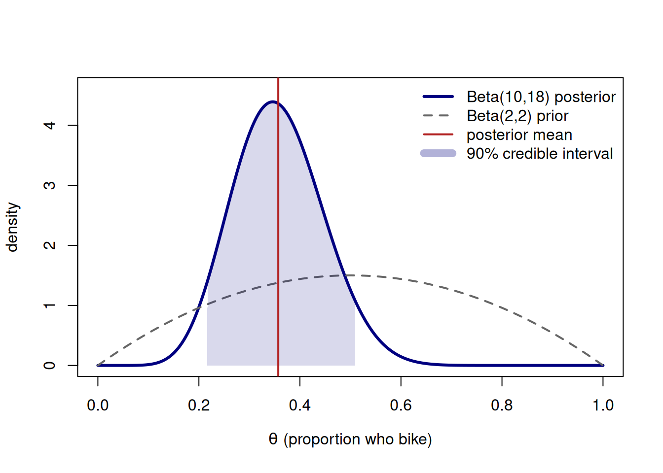
Move 4 — summarize and stress-test. Pair that mean with a 90% credible interval read off the Beta(10,18) quantiles (computed in the figure below, roughly 0.23 to 0.50). So our headline is: about 36% of students bike, plausibly between ~23% and ~50%. A quick sensitivity check — swapping the mild Beta(2,2) for a flat Beta(1,1) — gives Beta(9,17), mean \(9/26 \approx 0.346\): essentially the same story, so the conclusion is data-driven, not prior-driven.

Move 5 — predict and simulate. For a new class of, say, 10 students, the posterior predictive number of bikers is centered near \(10 \times 0.357 \approx 3.6\) but is wider than a plain Binomial because it carries our remaining uncertainty about \(\theta\). The figure below also draws 10,000 samples from Beta(10,18) to confirm the simulated mean and interval match the closed form.

set.seed(8)

# closed-form posterior summaries
ci <- qbeta(c(0.05, 0.95), 10, 18)   # 90% credible interval
post_mean <- 10 / 28

# draw the prior and posterior densities
theta <- seq(0, 1, length.out = 600)
prior <- dbeta(theta, 2, 2)
post  <- dbeta(theta, 10, 18)

plot(theta, post, type = "l", lwd = 3, col = "navy",
     xlab = expression(theta ~ "(proportion who bike)"),
     ylab = "density", ylim = c(0, max(post) * 1.05))
lines(theta, prior, lwd = 2, lty = 2, col = "gray40")

# shade the 90% credible interval under the posterior
inside <- theta >= ci[1] & theta <= ci[2]
polygon(c(ci[1], theta[inside], ci[2]),
        c(0, post[inside], 0),
        col = rgb(0, 0, 0.5, 0.15), border = NA)

abline(v = post_mean, lwd = 2, col = "firebrick")
legend("topright", bty = "n",
       legend = c("Beta(10,18) posterior", "Beta(2,2) prior",
                  "posterior mean", "90% credible interval"),
       col = c("navy", "gray40", "firebrick", rgb(0, 0, 0.5, 0.3)),
       lwd = c(3, 2, 2, 8), lty = c(1, 2, 1, 1))

# confirm simulation matches the closed form
draws <- rbeta(10000, 10, 18)
cat("closed-form mean:", round(post_mean, 3),
    "| simulated mean:", round(mean(draws), 3), "\n")

closed-form mean: 0.357 | simulated mean: 0.357 

cat("closed-form 90% CI:", round(ci, 3),
    "| simulated 90% CI:", round(quantile(draws, c(0.05, 0.95)), 3), "\n")

closed-form 90% CI: 0.217 0.509 | simulated 90% CI: 0.216 0.51 

Figure 1: Bike-to-campus, end to end: the mild Beta(2,2) prior, the Beta(10,18) posterior after 8 of 24 bikers, the posterior mean (~0.357), and a shaded 90% credible interval.

The printed lines make Move 5 concrete: the simulated mean and 90% interval land on the closed-form values, which is exactly the agreement you want to be able to produce and explain.

Worked example — clinic wait-time counts (transfer recap)

To prove the through-line is about the moves, not the Beta-Binomial in particular, run the same pipeline on a different model: estimating \(\lambda\), the average number of patients arriving per hour at a small clinic. This is the secondary recurring Gamma-Poisson case, and it follows the identical five steps.

Move 1 — prior. Past experience suggests a few arrivals per hour, so use \(f(\lambda) = \text{Gamma}(s, r) = \text{Gamma}(3, 1)\) (shape 3, rate 1), whose mean is \(s/r = 3\).

Move 2 — likelihood. We observe \(n = 4\) hours with arrival counts \(2, 5, 3, 4\), total \(\sum y = 14\). Counts use the Poisson model, giving a likelihood \(\propto \lambda^{\sum y}\, e^{-n\lambda}\).

Move 3 — posterior. Gamma-Poisson updating adds the total count to the shape and the number of observations to the rate: \[ \lambda \mid y \;\sim\; \text{Gamma}(s + \textstyle\sum y,\; r + n) \;=\; \text{Gamma}(3 + 14,\; 1 + 4) \;=\; \text{Gamma}(17, 5). \]

Move 4 — summarize. The posterior mean is \(17/5 = 3.4\) arrivals per hour, and we pair it with a credible interval from the Gamma quantiles (roughly 2.1 to 5.1). Headline: about 3.4 arrivals per hour, plausibly between ~2 and ~5.

Move 5 — predict. A posterior predictive for next hour’s count averages a Poisson(\(\lambda\)) over the Gamma(17,5) posterior — again wider than a plain Poisson because it carries our uncertainty about \(\lambda\). Notice that not one idea changed from the bike case: only the prior family and the data model did. That portability is what the midterm rewards.

A common mistake

The traps below are the recurring ones from Weeks 1–7 collected in one place — review them as a set, because a midterm tends to probe the seam between two of them.

• Treating the likelihood as a distribution over \(\theta\). \(L(\theta \mid y)\) is a function of \(\theta\) for fixed data; it need not integrate to 1 over \(\theta\) and is not “the probability of \(\theta\).” It only becomes a proper distribution after you multiply by the prior and normalize. Catch it: if you ever wrote “the probability that \(\theta = 0.4\) is the likelihood,” stop — that is a posterior statement, not a likelihood one.
• Reporting a point estimate alone. A posterior mean of 0.357 with no interval hides all the uncertainty. Catch it: never let a single number leave the page without a credible interval beside it.
• Calling a credible interval a confidence interval (or vice versa). A 90% credible interval is a direct probability statement about this \(\theta\) given the data; a confidence interval is a statement about the long-run coverage of the procedure. Catch it: if your sentence says “there is a 90% probability \(\theta\) is in here,” you mean credible — make sure your interval actually came from the posterior.
• Confusing the posterior with the posterior predictive. The posterior is about the parameter; the predictive is about a future observation. The predictive is wider. Catch it: ask “am I describing \(\theta\) or a future \(y\)?” before you state a number.
• Believing arithmetic over a model. Adding \(y\) and \(n-y\) to Beta shapes only works because we chose a Binomial likelihood and a Beta prior. Catch it: name the model before you do the bookkeeping.

Interpretation guidance

When you report “about 36% bike, 90% credible interval ~0.23 to 0.50,” here is what that does and does not mean.

• It does mean: given the mild Beta(2,2) prior, the 8-of-24 data, and the Binomial model, there is a 90% posterior probability that the true biking proportion lies between roughly 0.23 and 0.50, with the most central single guess near 0.357.
• It does not mean: that exactly 36% of this sample biked (that was \(8/24 \approx 0.333\), the raw rate — the posterior mean is pulled slightly toward the prior’s 0.5). It also does not mean the interval is a confidence interval, nor that the next class will have between 23% and 50% bikers — that future-sample question is the predictive, which is wider.
• It does carry its assumptions: change the prior to something strongly informative, or use a non-representative sample, and the number moves. The sensitivity check is what licenses the claim “data-driven.” Always report the model and prior alongside the headline so a reader can judge it.

The discipline is: a Bayesian result is a statement under a model, not a fact about the world. Saying the model out loud is part of saying the result correctly.

Practice (ungraded)

Check-your-understanding prompts — no answer keys here; work them, then test yourself against the worked examples above.

1. A new survey finds 5 bikers in 12 students. Starting from Beta(2,2), write the posterior and its mean. Is it closer to the raw rate \(5/12\) or to 0.5, and why?
2. In one sentence, explain what the \(\propto\) in \(f(\theta \mid y) \propto L(\theta \mid y)\,f(\theta)\) drops and why dropping it is safe.
3. You report a posterior mean of 0.40 with a 90% credible interval of (0.31, 0.49). A friend says “so there’s a 90% chance the procedure is right.” Diagnose the error and restate the sentence correctly.
4. For the clinic case, you observe one more hour with 6 arrivals. Update Gamma(17,5) to its new shape and rate and give the new posterior mean.
5. Without computing, say which is wider — the posterior for \(\theta\) or the posterior predictive for the next class’s biker count — and explain the reason in terms of “what each one is about.”
6. Sketch (in words) how you would simulate the Beta(10,18) posterior and check that the simulated 90% interval matches the closed-form one.

Reading guide

This week maps back across the whole spine rather than to one new chapter — use it as a re-reading plan keyed to where each move came from. From Bayes Rules! (Vitalk, Dogucu & Hu; CC BY-NC-SA 4.0): Chapter 1 grounds the plausibility-updating mindset behind Move 1; Chapter 2 is the discrete Bayes’ rule the central identity generalizes; Chapter 3 is the Beta-Binomial model that drives the bike case (Moves 1–3); Chapter 4 justifies the prior-sensitivity stress-test and the fact that update order does not matter (Move 4); Chapters 6–8 cover approximation, posterior summaries, and posterior prediction — the basis for credible-interval reporting and the predictive/simulation work in Moves 4–5. Re-read the chapter summaries first; dig into a section only where your self-check flagged a gap. The clinic transfer case follows the Gamma-Poisson logic in the spirit of Chapter 5’s other conjugate models — read it for the pattern, not the example.

Public vs. graded

These notes and the practice prompts are public and ungraded; no answer keys are posted here. The midterm itself — its exact prompts, format, weighting, rubric, point values, and date — lives in the LMS, and the LMS (Blackboard) is authoritative for every graded specific. If anything on this page seems to disagree with the LMS, the LMS wins.

Looking ahead

Next week, Week 9 — Bayesian regression I, the unknown stops being a single proportion and becomes a relationship: we put priors on the coefficients of \(y_i = \beta_0 + \beta_1 x_i + \varepsilon_i\) (think study-hours predicting exam-score) and read each coefficient’s posterior mean with its credible interval — the same five moves, now in more than one dimension.

See also

• Lab 7 — Grid approximation in Quarto — the simulation/approximation workflow this week leans on.
• Notation glossary — the symbols and distributions recalled above.
• Bayes vs. classical cheat-sheet — for the credible-vs-confidence contrast.
• Syllabus — course shape and the public/graded boundary.