Why a Beta prior and Binomial data give a Beta posterior, and how to read it
Mathematical goal
This week we make precise a claim that Week 3 only sketched: when we model an unknown proportion \(\theta\) with a Beta prior and observe Binomial data, the posterior is again a Beta distribution, and we can write down its parameters without doing a single integral. The goal is to derive that result by recognizing the kernel of a Beta density inside the product \(L(\theta \mid y)\, f(\theta)\), and then to read the resulting posterior responsibly — pairing a point summary with a credible interval.
Concretely, by the end you should be able to start from a Beta(\(\alpha,\beta\)) prior, observe \(y\) successes in \(n\) trials, and produce the posterior Beta(\(\alpha+y,\ \beta+n-y\)) together with its mean \((\alpha+y)/(\alpha+\beta+n)\) — and explain why each piece appears.
The week question
If we believe a proportion \(\theta\) lives somewhere on \([0,1]\) and then we watch \(y\) successes out of \(n\) tries, exactly which Beta distribution describes what we now believe about \(\theta\) — and how do we summarize it honestly?
Where we are and why this matters
In Week 3 we built the machinery of prior, likelihood, posterior on the recurring bike-to-campus survey: we want \(\theta\), the proportion of students who bike to campus, we encoded a starting belief as a prior \(f(\theta)\), and we let data reshape it through the central identity
That identity is true in general, but in general the proportionality constant — the evidence \(f(y)\) — requires an integral that we cannot always do by hand. This week we cash in a piece of good luck: for proportions, a Beta prior and a Binomial likelihood fit together so cleanly that the integral takes care of itself. This pairing is called conjugacy, and it is the first fully worked, closed-form Bayesian model in the course. Everything later (prior sensitivity in Week 5, prediction in Week 6, simulation in Week 7) builds on being able to write this posterior down exactly.
This matters because it turns Bayesian updating from an abstraction into arithmetic: “two new numbers” instead of “an intractable integral.”
Notation
This week leans on the fixed course notation. The table below is the working ledger; the words in it are the ones the derivation manipulates.
Symbol
Meaning
\(\theta\)
the unknown parameter — here a proportion in \([0,1]\)
\(y\)
observed data — the number of successes
\(n\)
the number of trials (fixed in advance)
\(f(\theta)\)
the prior pdf on \(\theta\)
\(L(\theta \mid y)\)
the likelihood — a function of \(\theta\), not a distribution over \(\theta\)
\(f(\theta \mid y)\)
the posterior pdf on \(\theta\)
\(f(y)\)
the evidence / marginal — the normalizing constant \(\propto\) drops
Beta(\(\alpha,\beta\))
Beta with shape-shape parameters \(\alpha,\beta>0\)
\(\propto\)
“proportional to”: equal up to a factor not depending on \(\theta\)
A reminder on parameterization that will matter below: we always write Beta(\(\alpha,\beta\)) in the shape-shape convention. Both \(\alpha\) and \(\beta\) are shapes; neither is a rate.
Conceptual setup
Before any algebra, recall the two ingredients and what we assume about each.
The prior. We assume \(\theta \sim\) Beta(\(\alpha,\beta\)). The Beta family is supported on \([0,1]\), which is exactly the home of a proportion, so it is a natural language for prior belief about \(\theta\). Its density is
where \(B(\alpha,\beta)\) is the Beta function, a constant that makes the density integrate to 1. The part that depends on \(\theta\) — the kernel — is \(\theta^{\alpha-1}(1-\theta)^{\beta-1}\). Hold onto that shape.
The likelihood. We assume the data model is Binomial: given \(\theta\), the count of successes \(Y\) in \(n\) independent trials each with success probability \(\theta\) has
Read as a function of \(\theta\) (with \(y\) and \(n\) fixed by the data), the \(\binom{n}{y}\) is just a constant. The kernel in \(\theta\) is \(\theta^{y}(1-\theta)^{n-y}\).
The setup is now suggestive: both kernels are powers of \(\theta\) times powers of \((1-\theta)\). When we multiply them, the exponents simply add. That is the whole trick.
The derivation by kernel recognition
Start from the central identity and substitute the two pieces, keeping only what depends on \(\theta\) (every constant gets absorbed into \(\propto\)):
Here \(\propto\) has dropped two things: the binomial coefficient \(\binom{n}{y}\) from the likelihood, and the Beta-function constant \(1/B(\alpha,\beta)\) from the prior — neither depends on \(\theta\), and the evidence \(f(y)\) (also a constant in \(\theta\)) is what would restore equality. Now combine the like bases by adding exponents:
Compare this to the Beta kernel \(\theta^{a-1}(1-\theta)^{b-1}\). It matches exactly, with
\[
a = \alpha + y, \qquad b = \beta + n - y.
\]
A density is determined by its kernel (the normalizing constant is forced once the kernel is fixed), so we can read off the answer without integrating:
\[
\boxed{\,\theta \mid y \;\sim\; \text{Beta}(\alpha + y,\ \beta + n - y).\,}
\]
This is conjugacy: a Beta prior plus Binomial data yields a Beta posterior. The update rule is almost embarrassingly simple — add your successes \(y\) to \(\alpha\), add your failures \(n-y\) to \(\beta\).
The posterior mean
The mean of a Beta(\(a,b\)) is \(a/(a+b)\). Plugging in our posterior shapes:
It is worth seeing this as a weighted average of the prior mean \(\alpha/(\alpha+\beta)\) and the data proportion \(y/n\):
\[
\frac{\alpha + y}{\alpha + \beta + n}
= \underbrace{\frac{\alpha+\beta}{\alpha+\beta+n}}_{\text{weight on prior}}\cdot\frac{\alpha}{\alpha+\beta}
\;+\;
\underbrace{\frac{n}{\alpha+\beta+n}}_{\text{weight on data}}\cdot\frac{y}{n}.
\]
As \(n\) grows, the weight on the data goes to 1 and the prior fades — the balance idea from Bayes Rules! Chapter 4. The quantity \(\alpha+\beta\) behaves like a “prior sample size”: a large \(\alpha+\beta\) is a confident prior that the data must work harder to move.
Credible intervals from the Beta posterior
A point estimate alone hides our uncertainty, so we always pair the posterior mean (or median) with a credible interval. A 95% credible interval is an interval \([\ell, u]\) such that
\[
P(\ell \le \theta \le u \mid y) = 0.95.
\]
For a Beta posterior the equal-tailed version is immediate from quantiles: take the 2.5th and 97.5th percentiles of Beta(\(\alpha+y,\ \beta+n-y\)). In R these are qbeta(0.025, a, b) and qbeta(0.975, a, b). We can also approximate the same interval by simulation — draw many values with rbeta and read off the empirical quantiles — which is the bridge to Week 7.
The interpretation is direct and is one of the genuine payoffs of the Bayesian framing: given the data and the model, there is a 95% posterior probability that \(\theta\) lies in the interval. That is a statement about \(\theta\), which is what we usually wanted all along.
Worked examples
We work two cases: the recurring bike survey (symbolic, then numeric) and a transfer case in a different context, to show the update is about structure, not the story.
Worked example — bike-to-campus proportion (symbolic, then numeric)
This is the recurring case. We model \(\theta\), the proportion of students who bike to campus.
Symbolic. Take a mild prior Beta(\(\alpha,\beta\)) = Beta(2, 2), which is symmetric and gently favors values near \(1/2\) without much conviction (prior sample size \(\alpha+\beta = 4\)). Suppose the survey yields \(y\) bikers out of \(n\) respondents. By the derived rule,
Numeric instance. Now put in the recurring numbers: \(y = 8\) bikers out of \(n = 24\) respondents (so \(n - y = 16\) non-bikers). The update adds successes to \(\alpha\) and failures to \(\beta\):
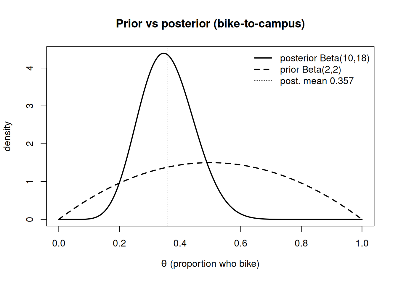
Compare the inputs: the prior mean was \(2/4 = 0.5\) and the raw data proportion was \(8/24 \approx 0.333\). The posterior mean \(0.357\) sits between them, pulled most of the way toward the data because \(n = 24\) outweighs the prior sample size of 4. The figure below shows the prior and the posterior together; the second figure shows the simulated posterior with its 95% credible interval shaded.
Figure 1: Prior Beta(2,2) and posterior Beta(10,18) for the bike-to-campus proportion. The posterior is tighter and centered near 0.357; the prior is broad and centered at 0.5.
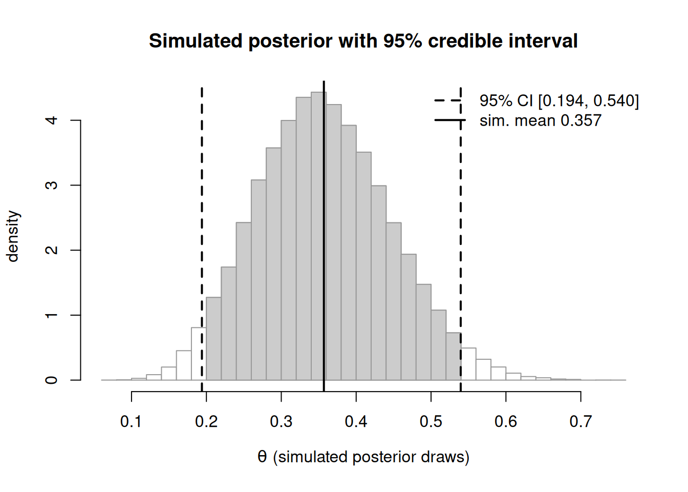
Figure 2: Simulated posterior draws for the bike proportion (50,000 rbeta draws from Beta(10,18)) as a histogram, with the equal-tailed 95% credible interval shaded and its endpoints from qbeta marked.
The simulated mean lands within rounding of the closed-form \(10/28 \approx 0.357\), and the shaded interval matches qbeta(c(0.025, 0.975), 10, 18) — a sanity check we will lean on in the lab.
Worked example — transfer case (sprouted seeds, a different proportion)
To show the update is about the structure, not the bikes, transfer it to a synthetic germination question: \(\theta\) is the proportion of seeds from a batch that sprout. We have no strong prior, so use a flat Beta(1, 1) (the uniform prior — every proportion equally plausible). We plant \(n = 40\) seeds and observe \(y = 30\) sprouts (\(n - y = 10\) duds).
Apply the same rule — successes onto \(\alpha\), failures onto \(\beta\):
With a flat prior the posterior mean \(31/42 \approx 0.738\) sits very close to the raw proportion \(30/40 = 0.75\); the tiny shift toward \(1/2\) is the residual pull of the Beta(1,1) “one prior success, one prior failure.” An equal-tailed 95% credible interval is qbeta(c(0.025, 0.975), 31, 11), roughly \([0.59, 0.86]\). We would report this as: “the posterior mean germination rate is about 0.74, 95% credible interval about \([0.59, 0.86]\)” — mean and interval, never the mean alone.
A convention warning
Three conventions cause most of the avoidable errors here; treat them as cautions.
Shape-shape, not shape-rate. Beta(\(\alpha,\beta\)) uses two shapes. Do not import the Gamma habit of treating the second argument as a rate. In R, dbeta(x, shape1, shape2), qbeta, and rbeta all expect the two Beta shapes in that order. Swapping them mirrors the distribution and silently corrupts every summary.
Credible interval is not a confidence interval. A 95% credible interval is a posterior probability statement about \(\theta\): given the data, \(P(\ell \le \theta \le u \mid y) = 0.95\). A frequentist 95% confidence interval is a statement about a procedure’s long-run coverage over hypothetical repeated samples, not a probability that this particular interval contains \(\theta\). They can even look numerically similar yet mean different things — never conflate them, and always say “credible interval” for a posterior.
What \(\propto\) drops. In the derivation, \(\propto\) discarded \(\binom{n}{y}\) and \(1/B(\alpha,\beta)\) and stood in for dividing by the evidence \(f(y)\). That is legitimate only because none of those depend on \(\theta\). If you ever drop something that does depend on \(\theta\), the kernel is wrong and so is the posterior.
Practice (ungraded)
Use these to check your understanding; no answer keys are posted here.
Starting from a Beta(3, 5) prior, you observe 12 successes in 20 trials. Write the posterior Beta parameters and its mean. Is the mean closer to the prior mean or the data proportion, and why?
In the bike example, suppose a second wave of the survey adds 5 more bikers out of 15 more respondents. Update the Beta(10, 18) posterior again (sequential updating). What single Beta would you have gotten by pooling all responses at once?
Explain, in one sentence each, what the \(\propto\) step is allowed to drop and what it is not allowed to drop.
Sketch (by hand or with curve(dbeta(x, 31, 11), 0, 1)) the germination posterior and mark roughly where its 95% credible interval falls.
A classmate reports “the posterior mean is 0.357” with no interval. Write the one extra thing they must report and why a point estimate alone is not enough.
Formula-verification status
These formulas are prepared as evidence but NOT yet human/source verified (verified: false); see the notation ledger. The course math gate is blocked pending sign-off. In particular, the conjugate update Beta(\(\alpha+y,\ \beta+n-y\)), the posterior mean \((\alpha+y)/(\alpha+\beta+n)\), and the credible-interval quantiles are staged here as derivation evidence; they should be treated as provisional until the math gate is cleared and a reviewer’s sign-off is recorded against the ledger.
Public vs. graded
This is a public, ungraded study note: no answer keys are posted here. Worked examples, practice prompts, and figures are for learning, not for credit. Anything graded — quiz items, their prompts and keys, weights, rubrics, point values, and due dates — lives in the LMS. The LMS (Blackboard) is authoritative for all of it. If this page and the LMS ever disagree, follow the LMS.
Looking ahead
Next week (Week 5 — Prior sensitivity & summaries) we hold the data fixed and ask how much the choice of Beta prior actually changes the posterior, and we sharpen how we summarize a posterior beyond the mean. See Week 5 — Prior sensitivity & summaries.