Week 5 — Prior sensitivity & summaries

When does the prior matter, when does it wash out, and how do we summarize the posterior honestly?

The week question

If two careful people start from different prior beliefs but see the same data, when do they end up agreeing — and how should we report a conclusion that we know depends on an assumption?

Where we are and why this matters

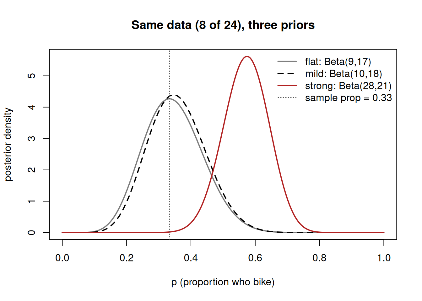
In Week 4 we built the Beta-Binomial model for an unknown proportion. The recurring case was the bike survey: a mild prior \(\text{Beta}(2,2)\) on \(p\), the proportion of students who bike to campus, combined with data of 8 bikers out of 24 surveyed, gave the posterior \(\text{Beta}(10,18)\) with posterior mean \(10/28 \approx 0.357\). That single posterior was the whole story last week.

This week we stop treating the prior as a fixed, unquestioned input and start treating it as an assumption we can vary. A skeptic might object: “you only got that answer because you chose that prior.” That objection is fair, and the honest response is not to defend one prior but to show what happens under several priors and report whether the conclusion holds up. Two ideas make this tractable. First, balance: the posterior is a compromise between the prior and the likelihood, and the relative weight depends on how strong the prior is versus how much data we have. Second, sequentiality: updating with all the data at once gives the same posterior as updating one batch at a time — so “more data” is just more updating, and we can watch a prior get overruled. Once we can produce a posterior under any prior, we also need a disciplined way to summarize it, which is the second half of the week: posterior mean versus median, and credible intervals versus predictive intervals.

Learning goals

By the end of this week you should be able to:

Re-compute the Beta-Binomial posterior under flat, mild, and strong priors with the same data, and explain why they differ.
Describe balance: how the prior’s strength and the sample size trade off in determining the posterior.
Use sequentiality to argue that accumulating data eventually overrules a reasonable prior — and say honestly when “eventually” has not yet arrived.
Choose and interpret a posterior point summary (mean vs. median) paired with a credible interval.
Distinguish a credible interval (about the parameter) from a predictive interval (about a future observation), and report a sensitivity analysis without overclaiming.

Core vocabulary

Prior strength. Informally, how much “prior data” a prior is worth. For a \(\text{Beta}(\alpha,\beta)\) prior, \(\alpha+\beta\) behaves like a prior sample size: bigger \(\alpha+\beta\) means a stronger, more stubborn prior.
Flat / mild / strong prior. A flat prior (e.g. \(\text{Beta}(1,1)\), uniform on \([0,1]\)) expresses little preference; a mild prior (e.g. \(\text{Beta}(2,2)\)) gently favors middle values; a strong prior (e.g. \(\text{Beta}(20,5)\)) encodes a confident belief that is hard to move.
Balance. The posterior sits between the prior and the data; its location depends on their relative weights.
Sequentiality. Updating in stages and updating all at once give the same posterior; order does not matter for the final result.
Prior sensitivity (robustness). How much the posterior conclusion changes when we change the prior. A conclusion is robust if reasonable priors agree.
Posterior summary. A short description of the posterior: a point estimate (mean or median) plus a credible interval.
Predictive interval. An interval for a future observation \(y_{\text{new}}\), not for the parameter \(\theta\). Wider than a credible interval because it includes sampling variability.

Balance: the posterior is a compromise

The Beta-Binomial update rule makes balance concrete. With a \(\text{Beta}(\alpha,\beta)\) prior and \(y\) successes in \(n\) trials, the posterior is \(\text{Beta}(\alpha+y,\ \beta+n-y)\), with posterior mean

\[ \mathbb{E}[p \mid y] \;=\; \frac{\alpha+y}{\alpha+\beta+n}. \]

Read that mean as a weighted average of the prior mean \(\frac{\alpha}{\alpha+\beta}\) and the sample proportion \(\frac{y}{n}\). The prior contributes a “pseudo-count” of \(\alpha+\beta\) and the data contribute \(n\). When the prior is weak relative to the sample (\(\alpha+\beta \ll n\)), the posterior mean sits close to the sample proportion; when the prior is strong (\(\alpha+\beta \gg n\)), the posterior mean stays near the prior mean. The posterior is never “the prior” or “the data” alone — it is always the compromise, and the mixing weights are \(\alpha+\beta\) versus \(n\).

This is why the same data can lead to visibly different posteriors: a flat prior barely tugs, a strong prior tugs hard. The first worked example makes that visible.

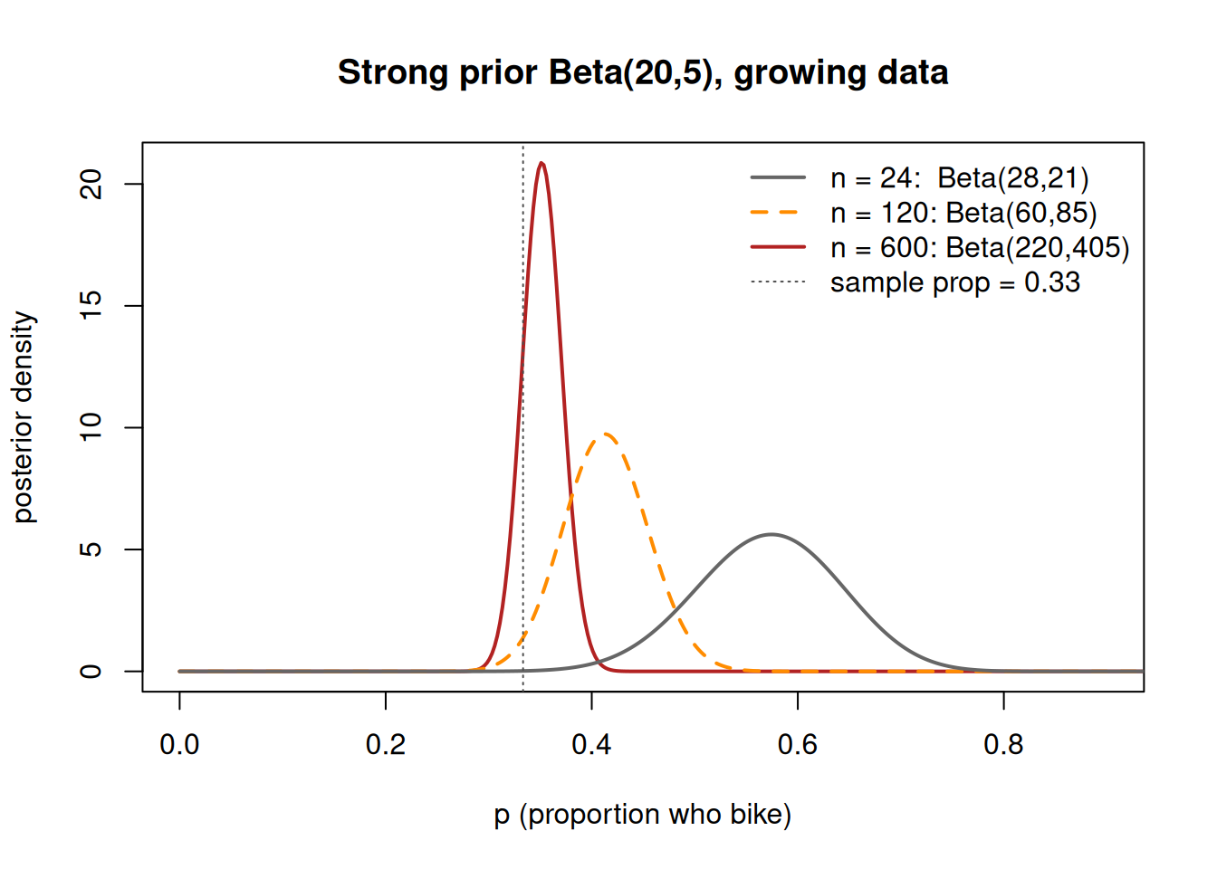
Sequentiality: more data eventually overrules the prior

Bayesian updating is sequential: today’s posterior is tomorrow’s prior. If you survey 12 students, form a posterior, then survey 12 more and update again, you land on exactly the same posterior as if you had pooled all 24 from the start. (For the Beta-Binomial this is easy to see: you just keep adding successes to \(\alpha\) and failures to \(\beta\), and addition does not care about order.)

The practical consequence is that the data’s pseudo-count \(n\) grows without bound while the prior’s \(\alpha+\beta\) stays fixed. So as \(n \to \infty\), the weight on the prior shrinks toward zero and the posterior mean is pulled toward the sample proportion. This is the precise sense in which “the data wash out the prior.” But notice the qualifier: it is an eventual statement. With a strong prior and a small sample, the prior can still dominate, and pretending otherwise is dishonest. The second worked example shows a strong prior surviving small data and only slowly giving way as data accumulate.

Summaries: mean vs. median, credible vs. predictive

Once you have a posterior, you report it, and three choices recur.

Point estimate: mean or median? The posterior mean is the balance point (sensitive to a long tail); the posterior median is the 50% point (robust to skew). For a roughly symmetric posterior they nearly coincide. For a skewed posterior — common when a proportion is near 0 or 1 — the median is often the more honest “typical value,” while the mean is the right summary if you will average or make an expected-value decision. Whichever you pick, never report a point alone: always pair it with a credible interval.

Credible interval. A 95% credible interval is an interval that holds 95% of the posterior probability for \(\theta\). You read it directly: “given the model and data, there is a 95% posterior probability that \(p\) lies in this range.” This is not the same claim as a frequentist confidence interval, whose 95% refers to the long-run coverage of the procedure, not the probability that the parameter is in this particular interval. We always say “credible interval” for a posterior and keep the two ideas apart.

Predictive interval. A credible interval is about the parameter \(p\). If instead you want a range for a future count — say, how many of the next 10 surveyed students will bike — you need a predictive interval, which adds the sampling variability of the new data on top of the parameter uncertainty. Predictive intervals are wider and answer a different question. (We develop posterior prediction fully in Week 6; here we only flag that a parameter interval and a prediction interval are not interchangeable.)

Worked example — Bike survey under three priors (recurring case)

Same data every time: 8 bikers of 24 surveyed. We compare three priors on \(p\).

Flat \(\text{Beta}(1,1)\) (prior mean \(0.500\)) \(\to\) posterior \(\text{Beta}(9,17)\), mean \(9/26 \approx 0.346\), 95% credible interval \([0.180,\ 0.535]\).
Mild \(\text{Beta}(2,2)\) (prior mean \(0.500\)) \(\to\) posterior \(\text{Beta}(10,18)\), mean \(10/28 \approx 0.357\), 95% credible interval \([0.194,\ 0.540]\).
Strong \(\text{Beta}(20,5)\) (prior mean \(0.800\)) \(\to\) posterior \(\text{Beta}(28,21)\), mean \(28/49 \approx 0.571\), 95% credible interval \([0.432,\ 0.705]\).

The flat and mild priors are weak (\(\alpha+\beta = 2\) and \(4\)) relative to \(n=24\), so both posteriors land near the sample proportion \(8/24 \approx 0.333\) and essentially agree. The strong prior (\(\alpha+\beta = 25\), worth more than the data) pulls the posterior up toward \(0.8\), and its credible interval barely overlaps the others. So the bike conclusion is robust to the choice between flat and mild priors but sensitive to an aggressive strong prior — exactly the kind of finding a sensitivity analysis is meant to surface. The figure overlays all three.

p <- seq(0, 1, length.out = 400)
flat   <- dbeta(p,  9, 17)
mild   <- dbeta(p, 10, 18)
strong <- dbeta(p, 28, 21)
plot(p, flat, type = "l", lwd = 2, col = "gray50",
     ylim = c(0, max(flat, mild, strong)),
     xlab = "p (proportion who bike)", ylab = "posterior density",
     main = "Same data (8 of 24), three priors")
lines(p, mild,   lwd = 2, lty = 2, col = "black")
lines(p, strong, lwd = 2, col = "firebrick")
abline(v = 8/24, lty = 3, col = "gray30")
legend("topright", bty = "n",
       legend = c("flat: Beta(9,17)", "mild: Beta(10,18)",
                  "strong: Beta(28,21)", "sample prop = 0.33"),
       col = c("gray50", "black", "firebrick", "gray30"),
       lwd = c(2, 2, 2, 1), lty = c(1, 2, 1, 3))

Plot of three Beta posterior density curves over p from 0 to 1. Two nearly overlapping curves (flat Beta(9,17) and mild Beta(10,18)) peak around 0.34 to 0.36. A third curve (strong, Beta(28,21)) peaks higher around 0.57 and is shifted to the right. A dashed vertical line marks the sample proportion at about 0.33. — Figure 1: Three posterior densities for the proportion of students who bike, all from the same data (8 of 24). The weak flat and mild priors give nearly identical posteriors near the sample proportion; the strong prior pulls the posterior noticeably upward.

Worked example — A strong prior washing out (recurring case continued)

Keep the strong prior \(\text{Beta}(20,5)\) and let the bike survey grow, holding the observed proportion fixed at roughly \(1/3\) to isolate the effect of sample size.

Data	Posterior	Posterior mean	95% credible interval
\(y=8,\ n=24\)	\(\text{Beta}(28,21)\)	\(0.571\)	\([0.432,\ 0.705]\)
\(y=40,\ n=120\)	\(\text{Beta}(60,85)\)	\(0.414\)	\([0.335,\ 0.495]\)
\(y=200,\ n=600\)	\(\text{Beta}(220,405)\)	\(0.352\)	\([0.315,\ 0.390]\)

At \(n=24\) the strong prior still dominates and the posterior mean (\(0.571\)) is far from the data’s \(1/3\). By \(n=120\) the data have begun to win, and by \(n=600\) the posterior mean (\(0.352\)) has essentially collapsed onto the sample proportion while the interval has tightened. This is sequentiality in action: the fixed prior pseudo-count of \(25\) is overwhelmed once \(n\) is large. The figure shows the three posteriors marching left toward the data.

p <- seq(0, 1, length.out = 400)
d1 <- dbeta(p,  28,  21)   # n = 24
d2 <- dbeta(p,  60,  85)   # n = 120
d3 <- dbeta(p, 220, 405)   # n = 600
plot(p, d3, type = "l", lwd = 2, col = "firebrick",
     xlim = c(0, 0.9), ylim = c(0, max(d1, d2, d3)),
     xlab = "p (proportion who bike)", ylab = "posterior density",
     main = "Strong prior Beta(20,5), growing data")
lines(p, d2, lwd = 2, lty = 2, col = "darkorange")
lines(p, d1, lwd = 2, col = "gray40")
abline(v = 1/3, lty = 3, col = "gray30")
legend("topright", bty = "n",
       legend = c("n = 24:  Beta(28,21)", "n = 120: Beta(60,85)",
                  "n = 600: Beta(220,405)", "sample prop = 0.33"),
       col = c("gray40", "darkorange", "firebrick", "gray30"),
       lwd = c(2, 2, 2, 1), lty = c(1, 2, 1, 3))

Plot of three Beta posterior density curves over p from 0 to 1. The n equals 24 curve is broad and centered near 0.57. The n equals 120 curve is narrower and centered near 0.41. The n equals 600 curve is the tallest and narrowest, centered near 0.35. A dashed vertical line marks the sample proportion at about 0.33. The curves shift left and sharpen as n increases. — Figure 2: The same strong prior Beta(20,5) updated with increasing amounts of data (at a fixed observed proportion near one third). As the sample grows, the posterior moves away from the prior’s belief and concentrates on the sample proportion.

Worked example — Transfer: a rare side effect with scarce data

Now move to a new context where a strong prior is legitimately influential because data are scarce. A clinic is monitoring a known-rare side effect of a treatment. Long experience says it occurs in roughly 6% of patients, encoded as a fairly strong prior \(\text{Beta}(2,30)\) (prior mean \(2/32 = 0.0625\)). A small pilot of 12 patients shows 1 affected.

With the informative prior: posterior \(\text{Beta}(3,41)\), mean \(\approx 0.068\), median \(\approx 0.062\), 95% credible interval \([0.015,\ 0.158]\).
With a flat prior \(\text{Beta}(1,1)\) and the same data: posterior \(\text{Beta}(2,12)\), mean \(\approx 0.143\), 95% credible interval \([0.019,\ 0.360]\).

Here the prior choice changes the conclusion a lot, and that is appropriate: with only 12 observations the data carry little weight, so well-justified prior knowledge should and does dominate. Notice also that this posterior is right-skewed (a proportion pinned near zero), so the median (\(0.062\)) is the more honest “typical value” than the mean (\(0.068\)) — a good case for preferring the median as the point summary. The lesson transfers from the bike case: prior sensitivity is not a flaw to hide but a property to report, and how much the prior matters depends on how much the data have to say.

A common mistake

Two opposite traps, both common:

“The prior is just bias, so a real analysis uses no prior.” A prior is an explicit, inspectable assumption — which is more honest than a hidden one, not less. Every analysis encodes assumptions; the Bayesian version writes them down where a skeptic can vary them. The right response to “your prior is biased” is to run the analysis under several priors and report the sensitivity, exactly as in the first worked example. A flat prior is also a choice, not the absence of one.

“More data always erases the prior, so the prior never really matters.” True only eventually. With small or noisy data and a strong prior, the prior can dominate the posterior — see the rare side-effect transfer case and the \(n=24\) row of the washout table. The way to catch this mistake is to actually check: compare \(\alpha+\beta\) (prior pseudo-count) to \(n\) (data count). If they are comparable or the prior is larger, the prior is still doing real work and you must say so.

Interpretation guidance

Report prior sensitivity honestly. A defensible write-up says: “Under a flat and a mild prior the posterior mean for the bike proportion is about 0.35 with a 95% credible interval of roughly \([0.18, 0.54]\); the conclusion is robust to that choice. Under a deliberately strong prior favoring high values the posterior mean rises to 0.57, so a reader who holds that strong prior would conclude differently.” That sentence does three correct things: it pairs a point estimate with a credible interval, it states which priors agree, and it names the assumption under which the conclusion would change.

What the result does not mean: a credible interval is not a confidence interval (the 95% is posterior probability about \(p\), not long-run coverage of a procedure); a credible interval is not a prediction interval for the next student (that is wider and is Week 6’s job); and a posterior that depends on the prior is not “wrong” — it is correctly reporting that the data alone did not settle the question. When reasonable priors disagree, the right conclusion is “we need more data,” not “pick the answer I like.”

Practice (ungraded)

Use these to check your understanding. No answers are posted here.

The bike data are \(8\) of \(24\). Under the prior \(\text{Beta}(2,2)\) the posterior is \(\text{Beta}(10,18)\). Without re-deriving, predict whether a \(\text{Beta}(4,4)\) prior would move the posterior mean closer to the sample proportion or further from it, and explain using the pseudo-count idea.
A colleague reports a posterior mean of \(0.571\) for the bike proportion and a sample proportion of \(0.333\). What does the gap tell you about their prior, and what single number would you ask for to judge whether the prior is doing too much work?
For a strongly right-skewed posterior near zero, you must report one point summary. Which would you choose, mean or median, and why? When would you switch to the other?
Explain in one or two sentences the difference between “a 95% credible interval for \(p\)” and “a 95% interval for the number of bikers among the next 10 students surveyed.” Which is wider, and why?
Sketch (by hand or in R) what the bike posterior would look like under a strong prior favoring a low proportion, e.g. \(\text{Beta}(5,20)\), with the same \(8\)-of-\(24\) data. Would the conclusion be robust across your flat, mild, and this low-favoring strong prior?

Reading guide

This week maps to Bayes Rules! Chapters 4 and 5.

Chapter 4 (balance & sequentiality) is the backbone of the first two worked examples. Read it for the idea that the posterior balances prior and data and that updating sequentially equals updating all at once. As you read, translate their balance discussion into our pseudo-count framing: prior weight \(\alpha+\beta\) versus data weight \(n\). The washout table is the chapter’s “more data eventually dominates” point made numeric on our bike case.
Chapter 5 (conjugate families) supports the mechanical ease of re-running the model under many priors: because the Beta is conjugate to the Binomial, every prior in our comparison stays a Beta and the update is just arithmetic. Use it to convince yourself that the three-prior comparison is cheap to produce — which is what makes a sensitivity analysis routine rather than heroic.

Read the concepts in your own words and keep our fixed notation; do not copy the book’s examples or datasets. The bike and side-effect cases here are course-original synthetic examples.

Public vs. graded

These notes and the ungraded practice above are the public, study-anywhere version of the week. Graded prompts, rubric values, point values, and due dates are not posted here. No answer keys are posted here, and for anything graded the LMS (Blackboard) is authoritative. If a graded item ever seems to disagree with a public page, follow the LMS.

Looking ahead

Next week (Week 6 — Posterior predictive thinking) we take the posterior we now know how to summarize and ask a new question: what does it predict about future data? That is where the predictive interval flagged above gets built properly.