Lab 4 — Beta-Binomial simulation

Simulate, summarize, and read a Beta posterior for the bike-to-campus proportion

Purpose. This lab puts the Week 4 derivation to work. You will simulate the Beta posterior for the bike-to-campus proportion, summarize it with a posterior mean and a 95% credible interval, and confirm the simulation agrees with the closed-form answer. Read it alongside Week 04 — The Beta-Binomial model.

The idea

The core concept is that the closed-form posterior and a simulated posterior are two views of the same object. Week 4 derived that a Beta(2,2) prior plus 8 bikers out of 24 gives a posterior Beta(10,18) with mean \(10/28 \approx 0.357\). Here we also obtain that posterior by drawing random values with rbeta, summarizing the draws, and checking that the simulated summaries match the formulas. Simulation matters because most real models later in the course have no clean closed form — we will only have draws — so learning to trust and read draws now pays off later.

Goal

Simulate a Beta posterior for the bike-to-campus proportion, summarize it (mean + 95% credible interval), and read the result — confirming the simulated mean matches the closed-form posterior mean \(10/28 \approx 0.357\).

Setup

First, make sure your local environment renders. If R, VS Code, or Quarto are not yet working, follow the R + VS Code + Quarto setup page before you start. Then, create a new .qmd file in your course folder (for example lab-04-mywork.qmd), paste the chunks below one at a time, and render after each so you catch errors early. Everything here uses base R only — no add-on packages — so there is nothing extra to install.

Steps

Step 1 — Set the model and the closed-form answer

We hard-code the recurring numbers and compute the closed-form posterior so we have a target to hit. Seeding is not needed yet (no randomness), but we set it now so the whole document is reproducible.

set.seed(404)

# Prior Beta(alpha, beta) and data
alpha <- 2; beta <- 2
y <- 8; n <- 24            # 8 bikers of 24 respondents

# Conjugate update: successes onto alpha, failures onto beta
a_post <- alpha + y        # 10
b_post <- beta + (n - y)   # 18

# Closed-form summaries
post_mean_cf <- a_post / (a_post + b_post)
ci_cf <- qbeta(c(0.025, 0.975), a_post, b_post)

c(a_post = a_post, b_post = b_post,
  post_mean_cf = post_mean_cf,
  ci_lo = ci_cf[1], ci_hi = ci_cf[2])

      a_post       b_post post_mean_cf        ci_lo        ci_hi 
  10.0000000   18.0000000    0.3571429    0.1940072    0.5396073

You should see a_post = 10, b_post = 18, and a posterior mean near 0.357.

Step 2 — Simulate the posterior

Now draw many values from the posterior Beta and summarize the draws. The simulated mean and the empirical 2.5%/97.5% quantiles should land on the closed-form values from Step 1.

draws <- rbeta(50000, a_post, b_post)

post_mean_sim <- mean(draws)
ci_sim <- quantile(draws, c(0.025, 0.975))

c(post_mean_sim = post_mean_sim,
  ci_lo_sim = ci_sim[1], ci_hi_sim = ci_sim[2])

  post_mean_sim  ci_lo_sim.2.5% ci_hi_sim.97.5% 
      0.3568848       0.1929175       0.5398263

Step 3 — Plot the simulated posterior with its credible interval

This figure is the deliverable’s centerpiece: a histogram of the draws with the 95% credible interval shaded and the posterior mean marked.

h <- hist(draws, breaks = 40, plot = FALSE)
plot(h, freq = FALSE, col = "white", border = "grey60",
     xlab = expression(theta ~ "(proportion who bike)"),
     ylab = "density",
     main = "Lab 4: simulated posterior with 95% credible interval")
in_ci <- h$mids >= ci_sim[1] & h$mids <= ci_sim[2]
rect(h$breaks[-length(h$breaks)][in_ci], 0,
     h$breaks[-1][in_ci], h$density[in_ci],
     col = "grey80", border = "grey60")
abline(v = ci_sim, lwd = 2, lty = 2)
abline(v = post_mean_sim, lwd = 2, lty = 1)
legend("topright",
       legend = c(sprintf("95%% CI [%.3f, %.3f]", ci_sim[1], ci_sim[2]),
                  sprintf("mean %.3f", post_mean_sim)),
       lty = c(2, 1), lwd = 2, bty = "n")

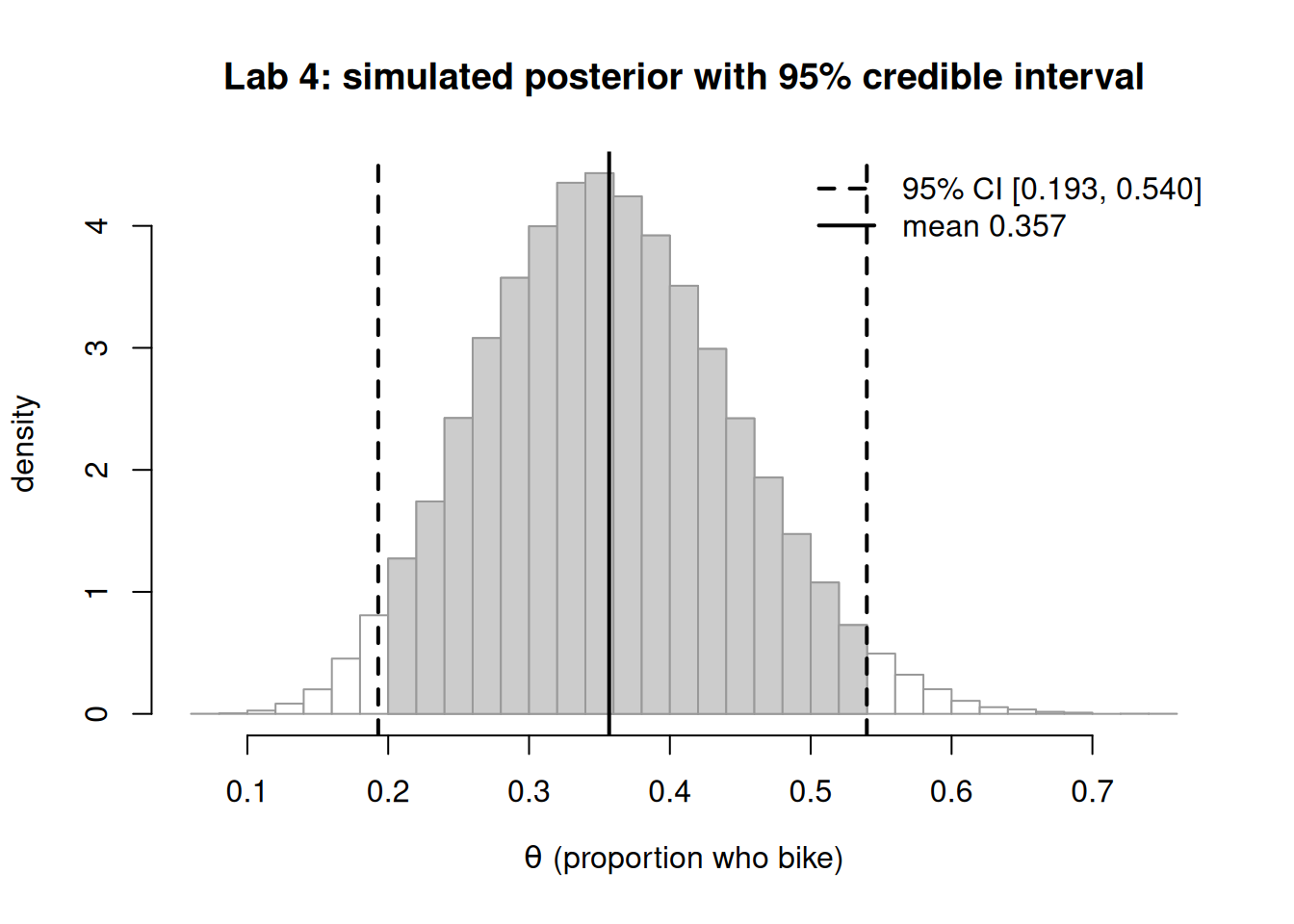
A density histogram of simulated bike-proportion values, mound-shaped and centered near 0.36. The central 95 percent of the mass is shaded between two dashed vertical lines at roughly 0.20 and 0.53, and a solid vertical line marks the posterior mean near 0.357. — Figure 1: Simulated posterior for the bike-to-campus proportion (50,000 draws from Beta(10,18)) with the equal-tailed 95% credible interval shaded and the posterior mean marked.

Step 4 — Overlay the exact density (optional check)

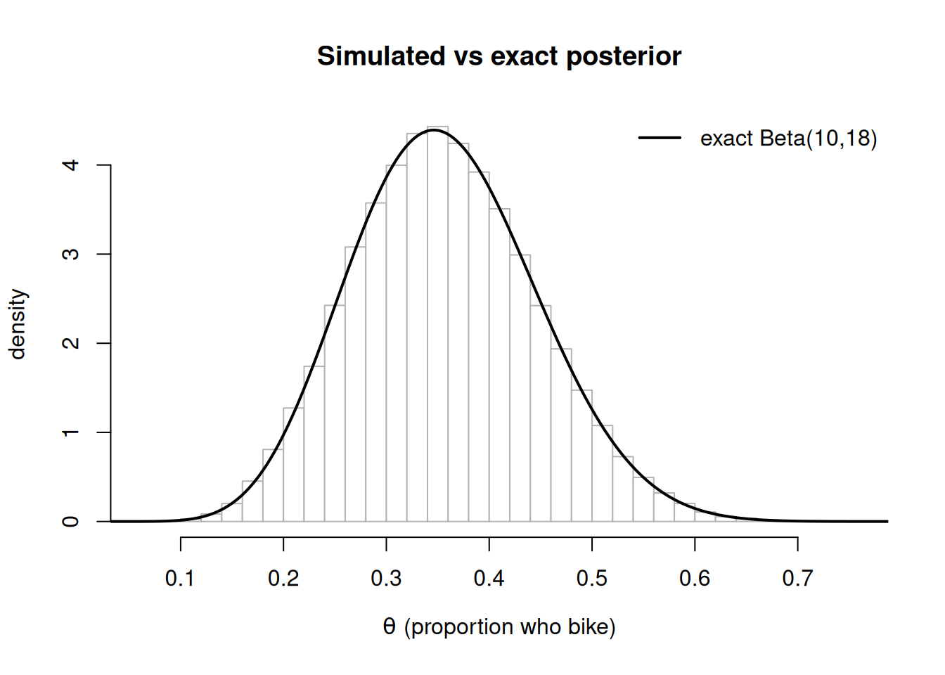
Adding the exact Beta(10,18) curve over the simulated density is a strong visual confirmation that the draws reproduce the closed-form posterior.

plot(h, freq = FALSE, col = "white", border = "grey70",
     xlab = expression(theta ~ "(proportion who bike)"),
     ylab = "density",
     main = "Simulated vs exact posterior")
xx <- seq(0, 1, length.out = 400)
lines(xx, dbeta(xx, a_post, b_post), lwd = 2)
legend("topright", legend = "exact Beta(10,18)", lwd = 2, bty = "n")

The same mound-shaped histogram of simulated bike-proportion values, with a smooth solid curve for the exact Beta(10,18) density drawn on top. The curve traces the top of the histogram bars almost exactly, showing the simulation matches the closed-form posterior. — Figure 2: Simulated posterior density (histogram) for the bike proportion with the exact Beta(10,18) density overlaid as a solid curve; the two agree closely.

Reproducible workflow

Keep the work tidy so it renders the same way for anyone (including future you):

Put all of this in a single .qmd file with a clear name (e.g. lab-04-mywork.qmd).
Call set.seed(404) once near the top so the simulation is reproducible on every render.
Save the file, then render the whole document end to end (not just chunk-by-chunk) to confirm it builds clean from a fresh state.
Use base R only; do not add library calls, so the .qmd renders on any machine with R.

When it breaks

A few common snags and fixes:

Render error: “could not find function rbeta”. You are almost certainly outside an R chunk or R is not on PATH. Confirm the chunk fence is {r} and recheck the setup page.
The shaded interval looks wrong / mirrored. You likely swapped the Beta shapes. Order is rbeta(n, shape1, shape2) = rbeta(n, a_post, b_post); if a_post and b_post are reversed, the distribution flips. Troubleshoot by printing c(a_post, b_post) and confirming 10, 18.
Simulated mean is noticeably off from 0.357. Either the seed/draw count changed or the data inputs are wrong. Increase draws to 50,000 and re-verify y = 8, n = 24. If a chunk fails, comment out everything below it, render, then re-add chunks one at a time to isolate the break.

A hands-on step

For the hands-on step, change one input and predict the result before you run it: set y <- 12 (keeping n <- 24), re-render, and check whether the posterior mean moved up toward 0.5 as you expected. This is the concrete activity carried into Lab 4 on the LMS.

Verify

Your lab succeeds if, in one render, all of the following hold:

The simulated posterior mean (post_mean_sim) agrees with the closed-form mean 10/28 = 0.357... to about two decimal places.
The simulated 95% interval (ci_sim) agrees with qbeta(c(0.025, 0.975), 10, 18) to about two decimal places.
The overlay in Step 4 shows the exact Beta(10,18) curve tracing the top of the histogram.

A compact numerical check you can include:

data.frame(
  quantity = c("posterior mean", "CI lower", "CI upper"),
  closed_form = c(post_mean_cf, ci_cf[1], ci_cf[2]),
  simulated   = c(post_mean_sim, ci_sim[1], ci_sim[2]),
  abs_diff    = abs(c(post_mean_cf, ci_cf[1], ci_cf[2]) -
                    c(post_mean_sim, ci_sim[1], ci_sim[2]))
)

            quantity closed_form simulated     abs_diff
      posterior mean   0.3571429 0.3568848 0.0002580525
2.5%        CI lower   0.1940072 0.1929175 0.0010896777
97.5%       CI upper   0.5396073 0.5398263 0.0002190004

All abs_diff values should be small (well under 0.01).

AI use note

Tool	Purpose	Verification
LLM assistant (optional)	explain an R error message or suggest a base-R idiom	Re-run the chunk yourself; confirm the simulated mean still matches `10/28` and the figure renders. Never paste a result you did not reproduce.

Use of an AI assistant is optional and never a substitute for running the code. Always verify any suggested code against the closed-form posterior before keeping it.