Why a positive test can still mean you probably don’t have the disease
The week question
If you take a test for a rare condition and it comes back positive, what is the probability you actually have the condition?
The honest answer surprises almost everyone: it can be low — sometimes well below 50% — even when the test is “95% accurate.” This week we build the machinery that explains why, and in doing so we meet Bayes’ rule in its cleanest, fully discrete form. Everything later in the course is a richer version of the move we make here.
Where we are and why this matters
In Week 1 we framed Bayesian thinking as plausibility updating: you start with what you believe about an unknown, you observe evidence, and you revise your belief so it accounts for that evidence. That was the idea. This week we make the idea mechanical and checkable in the simplest setting, where the unknown takes only a few discrete values and we can write every probability in a small table.
Discrete Bayes is the right place to start for two reasons. First, the arithmetic is fully visible — nothing is hidden inside an integral, so you can audit every number. Second, the diagnostic-test example forces a confrontation with base rates (how common the condition is before testing), which is exactly the ingredient people drop when they reason badly about evidence. Get the discrete case right and the continuous case in Week 3 is the same story with a smooth curve in place of a table.
Learning goals
By the end of this week you should be able to:
State conditional probability and read \(P(A \mid B)\) as “the probability of \(A\)given that\(B\) happened,” and explain why \(P(A \mid B)\) and \(P(B \mid A)\) are different quantities.
Write Bayes’ rule in discrete form and name each piece: prior, likelihood, marginal (evidence), posterior.
Define sensitivity, specificity, and base rate, and combine them to get the probability of disease given a positive test.
Solve a discrete updating problem two ways — as a counting table and via the Bayes’ rule formula — and check that they agree.
Diagnose base-rate neglect: spot when someone has confused \(P(\text{positive} \mid \text{disease})\) with \(P(\text{disease} \mid \text{positive})\).
Core vocabulary
Conditional probability\(P(A \mid B)\) — the probability of event \(A\) restricted to the world where \(B\) is true. Definition: \(P(A \mid B) = P(A \cap B) / P(B)\) when \(P(B) > 0\).
Prior — what you believe about the unknown before seeing this piece of evidence. In the diagnostic case the prior is the base rate, \(P(\text{disease})\).
Likelihood — how probable the evidence is under each value of the unknown. For a test, this is sensitivity and the false-positive rate.
Marginal probability (evidence) — the total probability of the evidence, summed over all values of the unknown. It is the normalizing piece \(f(y)\) that makes the posterior a valid probability.
Posterior — the updated belief about the unknown after the evidence, \(P(\text{disease} \mid
\text{positive})\).
Sensitivity — \(P(\text{positive} \mid \text{disease})\): among people who have the condition, the fraction the test correctly flags. (Also: true-positive rate.)
Specificity — \(P(\text{negative} \mid \text{no disease})\): among people who do not have it, the fraction the test correctly clears. (Its complement, \(1 - \text{specificity}\), is the false-positive rate.)
Base rate — the prior prevalence \(P(\text{disease})\) in the population being tested.
Conditional probability: the direction matters
The single most important idea this week is that a conditional probability has a direction, and flipping the direction changes the answer. \(P(\text{positive} \mid \text{disease})\) asks: among sick people, how many test positive? That is a property of the test. \(P(\text{disease} \mid \text{positive})\) asks: among people who tested positive, how many are sick? That is what a patient actually wants to know. These two are related but not equal, and the gap between them is where Bayes’ rule lives.
From the definition \(P(A \mid B) = P(A \cap B)/P(B)\), notice that \(P(A \cap B) = P(B \mid A)\,P(A)\). Substituting gives the discrete form of Bayes’ rule:
\[
P(A \mid B) \;=\; \frac{P(B \mid A)\, P(A)}{P(B)}.
\]
Read it as: posterior = (likelihood × prior) / evidence. The numerator reweights the prior \(P(A)\) by how well \(A\) explains the evidence \(B\); the denominator \(P(B)\) rescales so the result is a genuine probability. This is the discrete cousin of the course’s central identity \(f(\theta \mid y) \propto L(\theta \mid y)\, f(\theta)\) — the marginal \(P(B)\) (the \(f(y)\)) is exactly the constant that \(\propto\) would drop.
The evidence term is a weighted sum
The denominator \(P(B)\) rarely arrives handed to you. You build it by the law of total probability: split the world into the possible values of the unknown, find the probability of the evidence under each, and add. With a disease that is present (\(D\)) or absent (\(D^c\)):
The first term is true positives (sensitivity × base rate); the second is false positives (false-positive rate × the much larger non-diseased fraction). When the disease is rare, that second term can dominate — there are simply so many healthy people that even a small false-positive rate produces a flood of positive tests from people who are fine. That is the whole mystery in one line.
Sensitivity, specificity, base rate: putting them together
Three knobs control the answer: a higher base rate raises the posterior, higher sensitivity raises it, and higher specificity (fewer false positives) raises it. The base rate is the knob people forget — and it is often the most powerful one when the condition is rare.
Worked examples
The three cases below are the same machine run on different inputs: a rare-disease screen where the posterior is surprisingly low, the recurring bike-to-campus survey as a discrete table, and a spam filter where the posterior comes out high. Work each by hand and watch the base rate do its work.
Worked example — synthetic disease screening (table and Bayes’ rule)
Consider a synthetic screening scenario (numbers chosen for instruction, not from any real test or dataset):
Base rate: \(P(D) = 0.01\) (1 in 100 has the condition).
Specificity: \(0.90\), so the false-positive rate is \(P(\text{positive} \mid D^c) = 0.10\).
As a counting table. Imagine 10,000 people, which turns probabilities into whole-person counts you can add up:
Test positive
Test negative
Row total
Has condition (\(D\))
95
5
100
No condition (\(D^c\))
990
8910
9900
Column total
1085
8915
10000
Of the 100 diseased people, \(0.95 \times 100 = 95\) test positive. Of the 9900 healthy people, \(0.10 \times 9900 = 990\) test positive. So among the 1085 total positives, only 95 truly have the condition:
The two methods agree, as they must — the table is the formula, written out person by person. The headline: a “95% sensitive” test on a rare condition still leaves a positive person at under a 9% chance of actually having it. Most positives are false positives, because healthy people vastly outnumber sick ones.
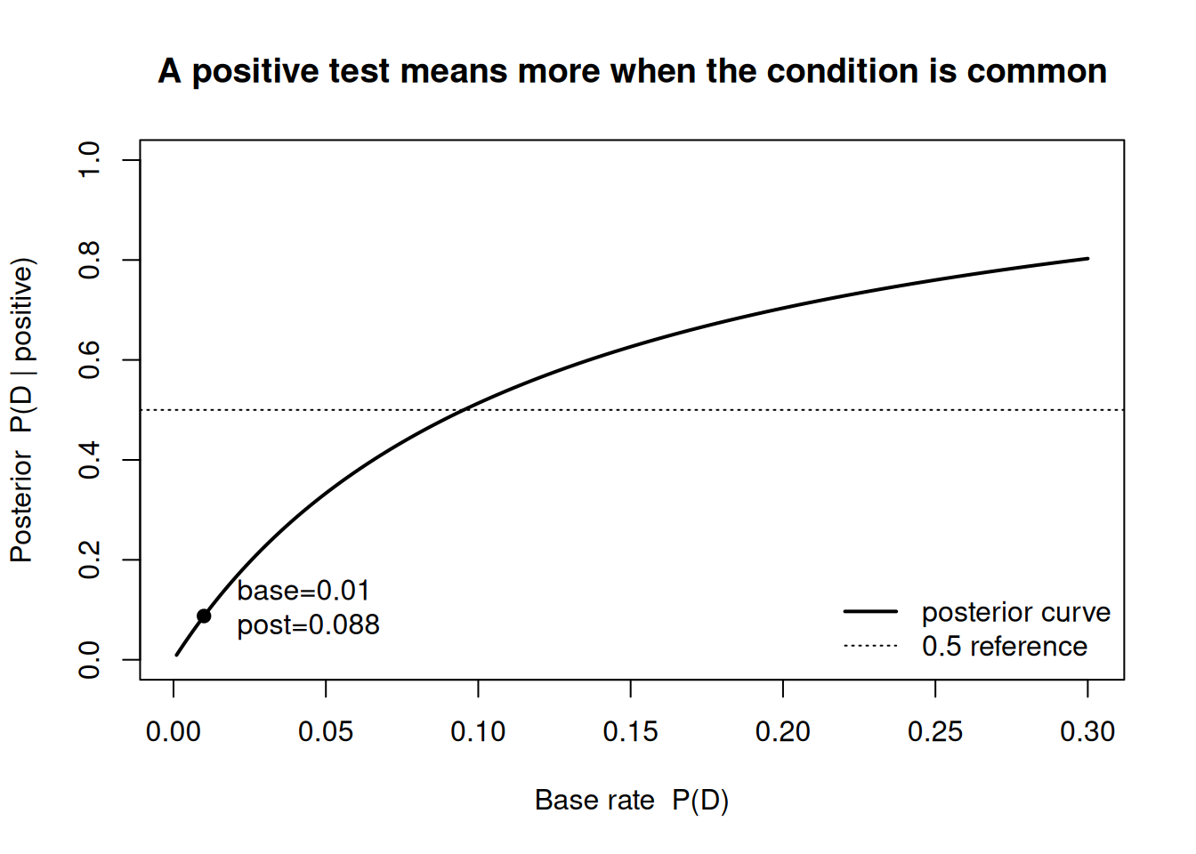
The figure below shows how the posterior \(P(D \mid \text{positive})\) climbs as the base rate climbs, holding sensitivity and specificity fixed at the values above.
sens <-0.95# sensitivity P(positive | D)fpr <-0.10# false-positive rate P(positive | not D)base <-seq(0.001, 0.30, length.out =400)post <- (sens * base) / (sens * base + fpr * (1- base))plot(base, post, type ="l", lwd =2,xlab ="Base rate P(D)",ylab ="Posterior P(D | positive)",main ="A positive test means more when the condition is common",ylim =c(0, 1))# mark the worked example at base rate 0.01b0 <-0.01p0 <- (sens * b0) / (sens * b0 + fpr * (1- b0))points(b0, p0, pch =19)text(b0, p0, labels =sprintf(" base=0.01\n post=%.3f", p0), pos =4)abline(h =0.5, lty =3)legend("bottomright", legend =c("posterior curve", "0.5 reference"),lwd =c(2, 1), lty =c(1, 3), bty ="n")
Figure 1: Posterior probability of the condition given a positive test, as a function of the base rate (prevalence), with sensitivity fixed at 0.95 and false-positive rate at 0.10. The dot marks the worked example at a 1% base rate.
Two lessons sit in this curve. The posterior is steeply sensitive to the base rate when the condition is rare (the left side), and it only crosses the 0.5 line once the condition is fairly common. Same test, very different meaning of a positive — entirely because of the prior.
Worked example — recurring case: bike-to-campus, discrete updating table
Now the course’s recurring question, in discrete form. We want the proportion\(p\) of students who bike to campus. Suppose, for this week only, that \(p\) can take just a few candidate values, and we hold a discrete prior over them (this is a coarse stand-in for the smooth Beta prior we adopt in Week 3). Our evidence is a tiny pilot: we ask 3 students and 1 of them bikes.
For each candidate \(p\), the likelihood of “1 biker out of 3” under independent responses is the binomial weight \(\binom{3}{1} p^1 (1-p)^2 = 3p(1-p)^2\). Because the \(\binom{3}{1} = 3\) is the same for every candidate, it cancels in Bayes’ rule — a first taste of “\(\propto\) drops constants.” The updating table:
Candidate \(p\)
Prior \(f(p)\)
Likelihood \(\propto p(1-p)^2\)
Prior × Likelihood
Posterior \(f(p \mid y)\)
0.2
0.20
0.128
0.02560
0.186
0.3
0.30
0.147
0.04410
0.320
0.4
0.30
0.144
0.04320
0.313
0.5
0.20
0.125
0.02500
0.181
The marginal (evidence) is the column sum of “Prior × Likelihood”: \(0.02560 + 0.04410 + 0.04320 + 0.02500 = 0.13790\). Dividing each entry by 0.13790 gives the posterior column above: \(0.02560/0.13790 \approx 0.186\), \(0.04410/0.13790 \approx 0.320\), \(0.04320/0.13790 \approx 0.313\), and \(0.02500/0.13790 \approx 0.181\) — and as a check, those four posterior weights sum to 1.
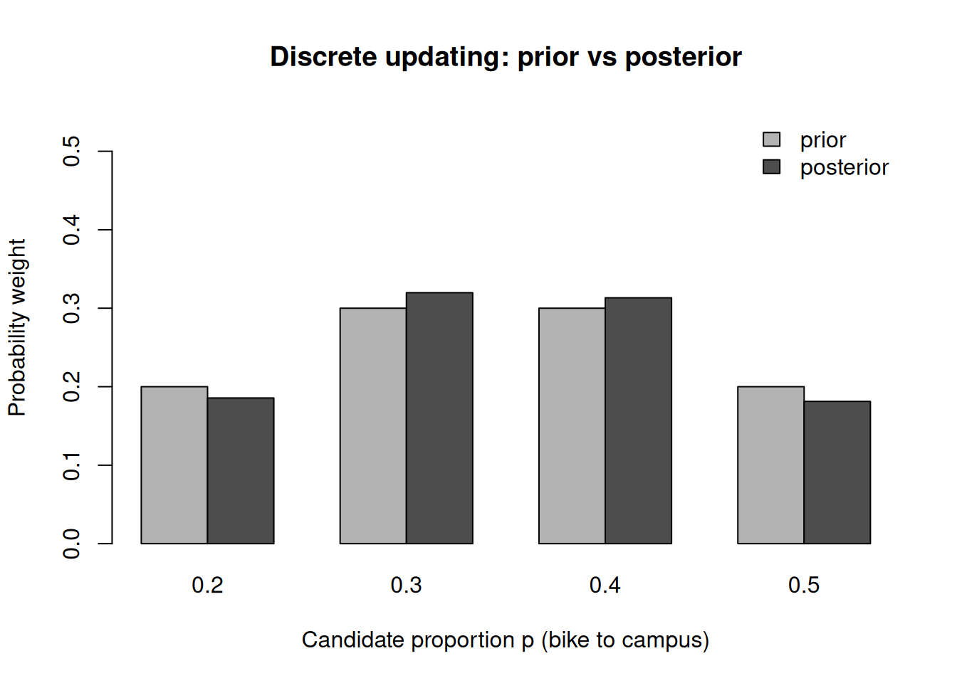
Notice the shape of the update: the prior favored \(p = 0.3\) and \(p = 0.4\) equally, and seeing 1 biker in 3 (an observed rate of \(0.33\)) concentrates a little more weight on the two candidates nearest that rate — both \(0.3\) and \(0.4\) rise above their prior, while the extremes \(0.2\) and \(0.5\) fall below theirs. The data nudged our belief; it did not overturn it, because three observations carry little weight. In Week 3 we let \(p\) range over the whole interval \([0,1]\) and replace this table with a Beta prior — and the same prior-times-likelihood logic produces the posterior Beta(10, 18) from the term’s recurring survey (prior Beta(2,2), 8 bikers of 24).
Figure 2: Discrete prior versus posterior over four candidate values of the bike-to-campus proportion, after observing 1 biker out of 3 surveyed. The posterior shifts mass slightly toward lower values.
Worked example — transfer case: spam filter (a positive flag)
The same arithmetic governs a context with nothing medical about it. A synthetic email filter flags messages as “spam.” Suppose 20% of incoming mail is genuinely spam (\(P(S) = 0.20\), the base rate). The filter flags 98% of true spam (\(P(\text{flag} \mid S) = 0.98\)) but also wrongly flags 3% of legitimate mail (\(P(\text{flag} \mid S^c) = 0.03\)). A message lands in your spam folder — how likely is it really spam?
Here the posterior is high — about 89% — because the base rate (20%) is far from tiny and the false-positive rate is low. Same formula, opposite feeling from the rare-disease case. The lesson transfers exactly: a positive flag is only as trustworthy as the base rate and the false-positive rate together allow.
A common mistake
The classic error this week is base-rate neglect: treating the test’s accuracy as if it were the probability of disease. A patient hears “the test is 95% accurate, and mine was positive,” and concludes “so I’m 95% likely to be sick.” That swaps \(P(\text{positive} \mid D)\) — a property of the test — for \(P(D \mid \text{positive})\) — what they actually want. The two differ by exactly the factor Bayes’ rule supplies, and when the base rate is small they differ enormously (95% versus under 9% in our worked example).
How to catch it. Whenever you see a conditional probability, say out loud which event is the “given.” If the quoted number conditions on disease status but the question asks about test result (or vice versa), you are about to flip a conditional and must run Bayes’ rule. A reliable gut-check: build the counting table for 10,000 people. If most of the positives come from the large healthy group, the posterior is low no matter how “accurate” the test sounds.
Interpretation guidance
A posterior like \(P(D \mid \text{positive}) \approx 0.09\) does not mean the test is broken or useless. It means a single positive on a rare condition is a reason to investigate further, not a diagnosis — which is precisely why real screening programs confirm positives with a second, independent test. (Re-running Bayes’ rule with the first posterior as the new prior, and a second positive as new evidence, drives the probability up sharply; that is Bayesian updating done twice.)
Equally, the number is conditional on the model inputs: the base rate, sensitivity, and specificity we assumed. Change the population (and thus the base rate) and the posterior changes even with the identical test. A posterior probability is always a statement given a prior and a likelihood — never a free-standing fact about the world. Carry that habit forward: in this course we will never report an estimate without being explicit about what it was conditioned on.
Practice (ungraded)
Use these to check your understanding. No solutions are posted here.
A synthetic test has sensitivity 0.90 and specificity 0.95. The base rate is 0.02. Build the 10,000-person counting table, then compute \(P(D \mid \text{positive})\) with Bayes’ rule, and confirm the two agree.
Holding sensitivity and specificity fixed, what base rate would push \(P(D \mid \text{positive})\) above 0.5? Reason from the curve in Figure 1 before computing.
In the bike-to-campus discrete table, finish the two missing posterior entries and verify the four posterior weights sum to 1. Which candidate gained the most weight, and why?
A friend says “the spam filter is 98% accurate, so anything in my spam folder is 98% likely to be spam.” Name the misconception and explain, in one sentence, what number they actually computed.
Suppose you get a second independent positive on the rare-disease test. Use your Week-2 posterior as the new prior and update again. Roughly how much does the probability move?
Reading guide
This week maps to Bayes Rules! Chapter 2 (Bayes’ Rule). Read it for the conditional-probability groundwork and the diagnostic-test framing; our worked numbers and the bike-to-campus table are course-original, so use the chapter for the concepts and this page for the running examples.
The chapter’s treatment of conditional probability and the difference between \(P(A \mid B)\) and \(P(B \mid A)\) underwrites our “Conditional probability: the direction matters” section — read it first.
Its development of Bayes’ rule (prior, likelihood, the normalizing/marginal term) maps onto “The evidence term is a weighted sum” and “Sensitivity, specificity, base rate” here. Pay attention to how the chapter builds the denominator by total probability — that is our weighted-sum point.
Where the chapter discusses how a test result revises a probability, connect it to both worked diagnostic examples and to the recurring discrete updating table — the table is the chapter’s logic rendered as counting.
Public vs. graded
These notes and the ungraded practice above are the public face of the week. The graded quiz for this week — its exact prompts, options, point values, rubric, and due date — lives in the LMS: the LMS (Blackboard) is authoritative for everything graded. No answer keys are posted here, and nothing on this page is a submission contract. Prepare from the worked examples and practice prompts; submit and be graded in Blackboard.
Looking ahead
Next week we let the unknown stop being a short list of candidates and become a continuous quantity. Week 3 — Prior, likelihood, posterior replaces this week’s discrete updating table with smooth prior and posterior densities, and shows how the very same prior-times-likelihood move produces a continuous posterior. The bike-to-campus table you built here becomes a Beta prior there.