Building a model from assumptions and data: posterior ∝ likelihood × prior
Mathematical goal
By the end of this week you should be able to take a question about an unknown quantity, turn it into three named mathematical objects — a prior, a likelihood, and a posterior — and show, with algebra you can check, how the data turns the first into the third. Concretely, the goal is to derive and defend the central identity of the course:
to say precisely what the proportionality symbol \(\propto\) drops, and to apply the identity in two settings: a discrete parameter (a short updating table, our bridge from Week 2) and a continuous parameter (a Beta prior on a proportion, our bridge into Week 4). The derivation is the deliverable; the numbers are there to let you check the algebra against arithmetic you can re-run.
Notation
The whole week lives or dies on keeping four objects distinct, so we name them first. This notation is inherited from the course notation glossary; nothing here overrides it.
Symbol
Reads as
What it is (and is not)
\(\theta\)
the parameter
the unknown we want to learn about (here, a proportion)
\(y\)
the data
what we actually observe
\(f(\theta)\)
the prior
a probability distribution over \(\theta\)before seeing \(y\)
\(L(\theta \mid y)\)
the likelihood
a function of \(\theta\) for the observed \(y\) — not a distribution over \(\theta\)
\(f(\theta \mid y)\)
the posterior
a probability distribution over \(\theta\)after seeing \(y\)
\(f(y)\)
the evidence
the normalizing constant (marginal likelihood); a number, not a function of \(\theta\)
\(\propto\)
“proportional to”
equality up to a constant that does not depend on \(\theta\)
Two of these rows are the ones reviewers trip on, so they get their own warnings later: \(L(\theta \mid y)\) is a function of \(\theta\), not a density over \(\theta\); and \(f(y)\) is a constant, not “another likelihood.” Keep capital \(P\) for events and lowercase \(f\) for densities throughout.
Conceptual setup
Here is the setup, stated as a recipe you can repeat for any problem this semester. To build a Bayesian model you must commit to three things, in this order.
First, recall what we already did in Week 2. There we had a discrete set of candidate values for the proportion of students who bike to campus — say the proportion could only be one of \(\{0.1, 0.2, 0.3, \ldots\}\) — and we filled in a table: a column of prior probabilities, a column of likelihoods, their product, and a final normalized column. That table is Bayes’ rule. This week we keep the exact same machine and let the parameter become continuous.
Second, we assume a generative story for the data — a model that says, “if the true value were \(\theta\), then data like \(y\) would arise with this probability.” That story, read as a function of \(\theta\) for the \(y\) we actually saw, is the likelihood \(L(\theta \mid y)\).
Third, we assume a prior \(f(\theta)\): an honest distribution describing what we believed about \(\theta\) before the data. The prior is a genuine probability distribution — it integrates to one over the range of \(\theta\).
The posterior is then forced on us by the rules of probability; we do not get to choose it. That is the point of the derivation below: given the prior and the likelihood, the posterior is not a matter of taste.
From Bayes’ rule for events to a rule for parameters
Bayes’ rule for two events \(A\) and \(B\) is the familiar \(P(A \mid B) = P(B \mid A)\,P(A) / P(B)\). Replace the event \(A\) with “the parameter takes value \(\theta\)” and the event \(B\) with “we observed data \(y\).” The pieces map across cleanly:
The denominator \(f(y)\) is the probability of the data averaged over every possible \(\theta\). For a continuous parameter that average is an integral,
and for a discrete parameter it is the corresponding sum, \(f(y) = \sum_{\theta} L(\theta \mid y)\, f(\theta)\) — which is exactly the “total” you computed at the bottom of the Week 2 table. The discrete-to-continuous switch is only this: a sum becomes an integral, and a pmf becomes a pdf. The logic does not change.
Why we usually drop the evidence: the \(\propto\) move
Notice that \(f(y)\) does not depend on \(\theta\) — once the data are in hand, it is a fixed number. So as a function of \(\theta\), dividing by \(f(y)\) only rescales the curve \(L(\theta \mid y)\, f(\theta)\); it never changes its shape. That is why we so often write
State what \(\propto\) drops: it drops the constant \(f(y)\) — and, more generally, any factor that does not involve \(\theta\). The shape of \(L(\theta \mid y)\,f(\theta)\)is the shape of the posterior; the dropped constant is just whatever number makes the area under that shape equal to one. We recover it at the end by integrating, or — in the lucky “conjugate” cases of the next two weeks — by recognizing the shape as a named distribution whose constant we already know.
This is liberating in practice. To find the posterior you can ignore the integral, multiply prior by likelihood, simplify the part that depends on \(\theta\), and only then ask “what distribution has this shape?” The hard integral \(f(y)\) is handled for free by the recognition step.
Worked example — symbolic: a Beta prior meets a Binomial likelihood (bike-to-campus)
Take our running case: \(\theta\) is the unknown proportion of students who bike to campus. We survey \(n\) students independently and count \(y\) bikers. The natural data model is Binomial: for a fixed \(\theta\),
Read this as a function of \(\theta\) (the \(y\) and \(n\) are now fixed numbers). The factor \(\binom{n}{y}\) does not contain \(\theta\), so it will be swept into the \(\propto\) constant in a moment.
For the prior, we want a distribution that lives on \([0,1]\) and whose shape we can tune. The Beta family does exactly that. With prior \(\theta \sim \text{Beta}(\alpha,\beta)\) in the shape–shape parameterization,
Here the \(\propto\) has dropped two constants that contain no \(\theta\): the binomial coefficient \(\binom{n}{y}\) and the Beta function \(B(\alpha,\beta)\) — and, implicitly, the evidence \(f(y)\). Collect exponents:
This is the kernel of a Beta distribution. We recognize the shape, so we know the constant for free:
\[
\boxed{\;\theta \mid y \;\sim\; \text{Beta}\big(\alpha + y,\ \beta + n - y\big).\;}
\]
The update rule is just bookkeeping: add the successes \(y\) to \(\alpha\), add the failures \(n-y\) to \(\beta\). This is the Beta-Binomial model we will study in full next week; today the point is that we derived it from \(\propto\) and a shape match, not by memorizing it.
Worked example — numeric instance: Beta(2,2) prior, 8 of 24 (re-run this)
Use a mild, gently informative prior \(\text{Beta}(2,2)\) — symmetric, centered at \(0.5\), a soft “probably somewhere in the middle, but I’m not sure.” Suppose the survey returns \(y = 8\) bikers out of \(n = 24\) students. Plug into the boxed rule:
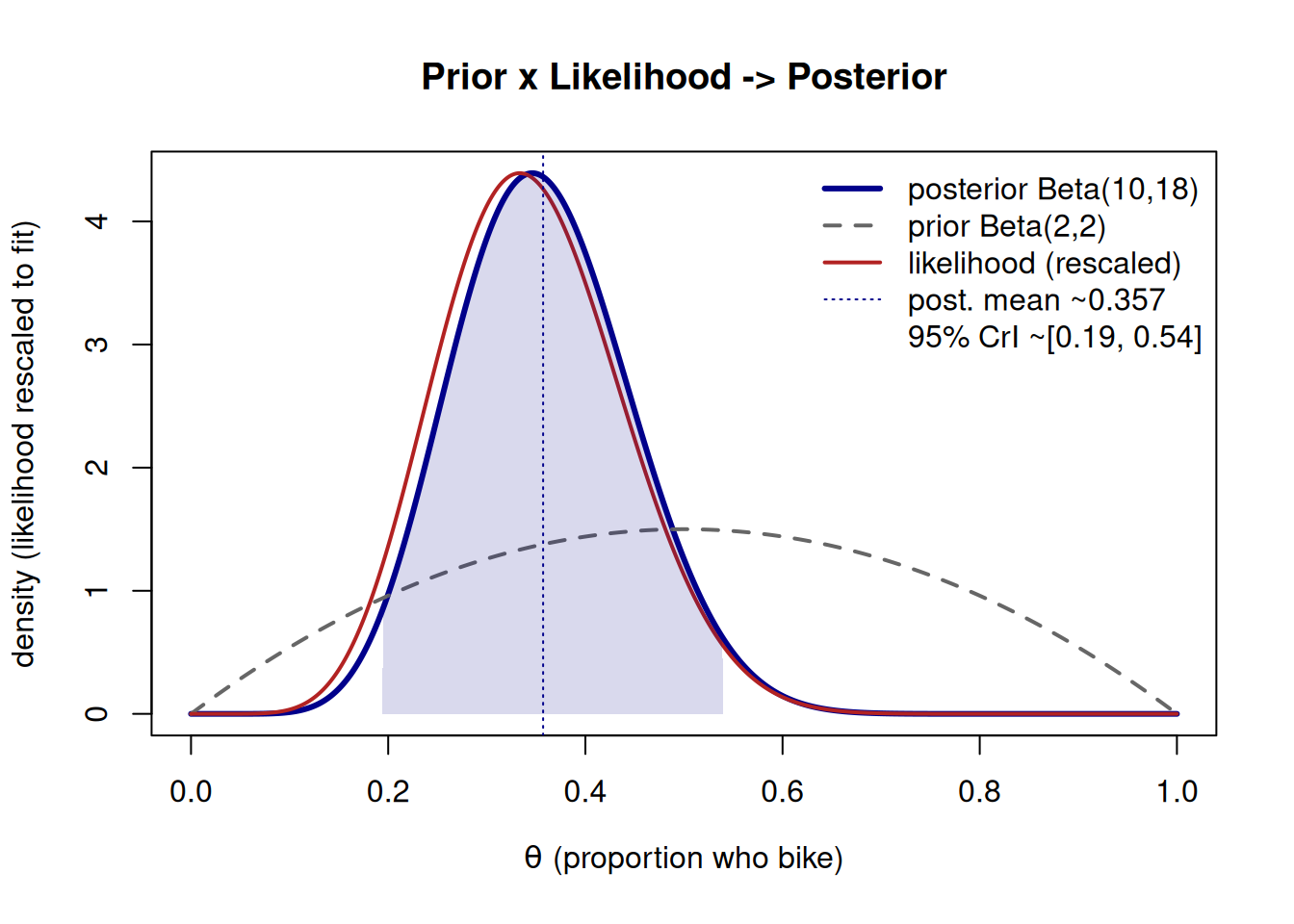
Sanity-check the direction. The prior mean was \(2/(2+2) = 0.5\). The data proportion was \(8/24 \approx 0.333\). The posterior mean \(0.357\) lands between them and is pulled most of the way toward the data — exactly what we expect, because \(n=24\) carries more weight than the \(\alpha+\beta = 4\) “prior sample size.” Pairing the point estimate with spread (a habit we never break): a central 95% credible interval here runs roughly from about \(0.20\) to about \(0.53\); the figure below reports it from the same posterior. Never quote the \(0.357\) alone.
The figure overlays the three actors on one axis so you can see the posterior sit between prior and likelihood.
set.seed(303)theta <-seq(0, 1, length.out =1001)# prior, posterior (true Beta densities)prior_d <-dbeta(theta, 2, 2)post_d <-dbeta(theta, 10, 18)# Binomial likelihood as a FUNCTION of theta (y = 8, n = 24).# Rescale only so it is visible on the same axis as the densities;# rescaling does not change its shape (this is the proportionality point).lik <- theta^8* (1- theta)^(24-8)lik_scaled <- lik /max(lik) *max(post_d)plot(theta, post_d, type ="l", lwd =3, col ="darkblue",xlab =expression(theta ~"(proportion who bike)"),ylab ="density (likelihood rescaled to fit)",main ="Prior x Likelihood -> Posterior")lines(theta, prior_d, lwd =2, lty =2, col ="gray40")lines(theta, lik_scaled, lwd =2, col ="firebrick")# posterior 95% credible intervalci <-qbeta(c(0.025, 0.975), 10, 18)inside <- theta >= ci[1] & theta <= ci[2]polygon(c(ci[1], theta[inside], ci[2]),c(0, post_d[inside], 0),col =rgb(0, 0, 0.55, 0.15), border =NA)abline(v =10/28, lty =3, col ="darkblue")legend("topright", bty ="n",legend =c("posterior Beta(10,18)", "prior Beta(2,2)","likelihood (rescaled)", "post. mean ~0.357",sprintf("95%% CrI ~[%.2f, %.2f]", ci[1], ci[2])),col =c("darkblue", "gray40", "firebrick", "darkblue", NA),lwd =c(3, 2, 2, 1, NA), lty =c(1, 2, 1, 3, NA))
Figure 1: Prior Beta(2,2), the rescaled Binomial likelihood for 8 of 24, and the resulting posterior Beta(10,18) for the bike-to-campus proportion. The posterior compromises between prior and data and is narrower than either.
The posterior is taller and narrower than the prior: 24 observations bought us real precision. That visible narrowing is what “learning from data” looks like.
Worked example — transfer: a discrete coin-bias table (no Beta needed)
To see that the logic is the same with sums instead of integrals, leave the bike case and consider a coin whose bias \(\theta\) we believe takes only one of three values, with a discrete prior:
\(\theta\)
prior \(f(\theta)\)
\(L(\theta \mid y)\) for \(y=2\) heads in \(n=3\)
\(L \cdot f\)
\(0.3\)
\(0.5\)
\(\binom{3}{2}(0.3)^2(0.7)^1 = 0.189\)
\(0.0945\)
\(0.5\)
\(0.3\)
\(\binom{3}{2}(0.5)^2(0.5)^1 = 0.375\)
\(0.1125\)
\(0.7\)
\(0.2\)
\(\binom{3}{2}(0.7)^2(0.3)^1 = 0.441\)
\(0.0882\)
The evidence is the column total, \(f(y) = 0.0945 + 0.1125 + 0.0882 = 0.2952\). Divide each \(L \cdot f\) by it to normalize:
Same three actors, same identity \(f(\theta \mid y) \propto L(\theta\mid y) f(\theta)\); the only difference from the bike case is that here \(f(y)\) is a sum over three values rather than an integral over \([0,1]\). That is precisely the bridge from Week 2’s table to this week’s continuous model.
A convention warning
Two cautions, both about reading symbols correctly — these are exactly the conventions a careless reader violates.
The likelihood is not a distribution over \(\theta\). It is tempting to look at \(L(\theta \mid y) = \binom{n}{y}\theta^y(1-\theta)^{n-y}\), see \(\theta\) varying, and treat it as a probability density for \(\theta\). It is not. As a function of \(\theta\) it does not integrate to one, and its area has no probabilistic meaning. The \(\theta\) in \(L(\theta \mid y)\) is a knob we turn to ask “how compatible is this\(\theta\) with the data we saw?” — not a random variable with its own distribution. Only after multiplying by the prior and normalizing do we obtain something that is a genuine distribution over \(\theta\): the posterior.
State what \(\propto\) drops, every time. The proportionality symbol is a promise that we have discarded only constants free of \(\theta\). In the symbolic example those were \(\binom{n}{y}\), \(B(\alpha,\beta)\), and the evidence \(f(y)\). If you ever “drop” something that secretly contains \(\theta\), the shape is wrong and the posterior is wrong. The discipline — caution as convention — is to write the \(\propto\) line and name the dropped factor in the same breath.
Practice (ungraded)
Use these to check your understanding; they are for practice only and have no posted answers.
In words, what does \(f(y) = \int L(\theta \mid y) f(\theta)\, d\theta\) compute, and why does it not depend on \(\theta\) once the data are fixed?
Start from \(\theta \sim \text{Beta}(2,2)\) and a different dataset, \(y = 5\) of \(n = 10\). Write the unnormalized posterior, then identify the Beta posterior and its mean. Is the mean pulled toward the data or the prior, and why?
Explain, to a classmate who missed lecture, why \(L(\theta \mid y)\) is not a probability distribution over \(\theta\). Give the one-sentence test you would use.
In the discrete coin table, what would change in the procedure if \(\theta\) could take five values instead of three? What stays exactly the same?
Rewrite the curve in Figure 1 in your own words: which curve is narrowest, and what does its narrowness say about how much the data taught us?
Formula-verification status
These formulas are prepared as evidence but NOT yet human/source verified (verified: false); see the notation ledger. The course math gate is blocked pending sign-off. Specifically, the central identity \(f(\theta \mid y) \propto L(\theta \mid y) f(\theta)\), the Beta-Binomial update \(\text{Beta}(\alpha+y,\ \beta+n-y)\), and the numeric instance \(\text{Beta}(2,2) \to \text{Beta}(10,18)\) with mean \(\approx 0.357\) are carried as re-derivations plus a numeric check, not as a self-certified result. None of this page is promotable past draft until a human/source sign-off is recorded in the ledger.
Reading guide
Bayes Rules! Ch 2 (Bayes’ Rule) reinforces the prior → likelihood → posterior structure built above and the role of the evidence \(f(y)\) as the normalizing constant we drop when we write \(\propto\). Read it after this week’s setup to see the same identity in the text’s framing.
Bayes Rules! Ch 3 (the Beta-Binomial model, intro) is where the continuous Beta prior we just put on the bike-to-campus proportion becomes a full conjugate model. Skim it now; we derive it in Week 4.
The notes are the spine; the reading reinforces and extends them — read by chapter, not cover to cover.
Public vs. graded
This is a public, ungraded study note. For anything graded, the LMS (Blackboard) is authoritative — weights, due dates, exact prompts, rubrics, and keys live there. No answer keys are posted here, and the practice prompts above are for self-study only.
Looking ahead
Next week — Week 4, The Beta-Binomial model — we stop treating the boxed update \(\text{Beta}(\alpha+y,\ \beta+n-y)\) as a one-off and study the whole conjugate family: why the Beta prior and Binomial likelihood fit together so neatly, how to choose \((\alpha,\beta)\) to encode a belief, and how to summarize the posterior with a mean and a credible interval you can defend.