Week 6 — Many-group comparisons & one-way ANOVA

Comparing several groups at once without inflating the error rate

The week question

Last week you compared two groups — Support versus Self-guided — and the whole apparatus had a clean shape: one difference in means, one standard error, one confidence interval, one effect size. This week the data structure changes in a way that looks like a small step and is actually a different problem. The Cypress Ridge redesign offered the quantitative-reasoning course in four instructional formats — Lecture (L), Lecture+Lab (LL), Online (O), and Hybrid (H) — and you have a final exam score for \(25\) students in each. The question is no longer “do these two differ?” but: do the four format means differ at all, and how do you ask that as one question instead of as a pile of pairwise questions?

Walking the analysis blueprint makes the shape obvious. The question is comparison — across more than two groups. The structure has a quantitative response (final score), one categorical grouping factor with four levels (format), \(n = 25\) per group in an observational setting (students were not randomly assigned to formats). The method that matches “one quantitative response, one factor with several levels” is one-way analysis of variance (ANOVA). The naive alternative — run a two-sample \(t\)-test on every pair of formats — feels natural and is a trap, and seeing exactly why it is a trap is the spine of this week. ANOVA replaces the pile of pairwise tests with a single omnibus test that asks one honest question while holding the error rate where you set it.

Why this matters

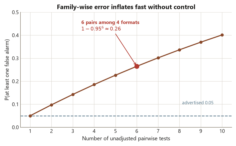
The reason a single omnibus test matters is not aesthetic tidiness; it is error-rate control, and it is the first place in the course where the act of asking many questions at once changes what an answer means. With four formats there are \(\binom{4}{2} = 6\) distinct pairs you could compare. If you test each pair at the \(5\%\) level and the formats are in truth identical, each test still has a \(5\%\) chance of a false alarm. Run six of them and the chance that at least one fires by luck climbs to roughly \(1 - (1 - 0.05)^6 \approx 0.26\) — about one in four. You set out to work at a \(5\%\) error rate and quietly ended up near \(26\%\). That gap between the rate you advertised and the rate you actually ran at is family-wise error inflation, and it is the disease the week is built around.

This matters for the same reason the whole course matters: a method is a way to connect a question to a data structure to an honest conclusion, and “honest” has a precise meaning here. A one-way ANOVA lets you ask “is there any format effect?” once, at the rate you chose, before you go looking at individual pairs. It also delivers what this course insists every analysis deliver — not a bare verdict but an estimate of how much: the effect size \(\eta^2\), the share of score variance that format explains. And it draws a bright line you must respect: a significant omnibus \(F\) tells you some formats differ; it does not tell you which. That second question — which pairs differ, controlled for multiplicity — is week 8’s job, and conflating the two is the classic error below. Keep estimate separate from verdict, and keep “something differs” separate from “these two differ,” and the week does its work.

Learning goals

By the end of this week you should be able to:

• State why running all pairwise \(t\)-tests inflates the family-wise error rate, and explain the one-way ANOVA as the single omnibus test that controls it.
• Identify the structure that calls for one-way ANOVA — one quantitative response, one categorical factor with three or more levels — using the blueprint, and say why ANOVA and not a pile of \(t\)-tests.
• Build a one-way ANOVA table from group means and sample sizes: the between- and within-group sums of squares, their degrees of freedom, the mean squares, and the \(F\)-ratio \(F = \mathrm{MS}_{\text{between}}/\mathrm{MSE}\).
• Report the analysis as an estimate with its uncertainty — the \(F\)-statistic and \(p\)-value plus the effect size \(\eta^2\) — and interpret \(\eta^2\) as the proportion of response variance explained by the factor.
• Say precisely what a significant \(F\) does and does not license: that some difference exists (not which groups), and that an observational design buys association, not causation.

Core vocabulary

• One-way ANOVA — the analysis matching one quantitative response and a single categorical factor with two or more levels; it partitions the total variation in the response into a part between group means and a part within groups, and compares the two.
• Grouping factor / levels — the categorical explanatory variable (here format) and its categories (L, LL, O, H). One factor, four levels, is the “one-way” in one-way ANOVA.
• Grand mean \(\bar{\bar x}\) — the mean of all \(N\) observations pooled across groups; the reference point against which each group mean is measured.
• Between-group sum of squares \(\mathrm{SS}_{\text{between}}\) — how far the group means sit from the grand mean, weighted by group size: \(\sum_j n_j(\bar x_j - \bar{\bar x})^2\). It is the signal — variation the factor could explain.
• Within-group sum of squares \(\mathrm{SS}_{\text{within}}\) — how far individual scores sit from their own group mean: \(\sum_j \sum_i (x_{ij} - \bar x_j)^2\). It is the noise — variation the factor cannot explain.
• Mean square — a sum of squares divided by its degrees of freedom; \(\mathrm{MS}_{\text{between}}\) on \(k - 1\) df, the within-group mean square \(\mathrm{MSE}\) on \(N - k\) df. Each is a variance.
• \(F\)-ratio — \(F = \mathrm{MS}_{\text{between}}/\mathrm{MSE}\): signal variance over noise variance. Under the null of equal means it is near \(1\); a large \(F\) is evidence some means differ.
• \(\eta^2\) (eta-squared) — the effect size: \(\eta^2 = \mathrm{SS}_{\text{between}}/ \mathrm{SS}_{\text{total}}\), the proportion of total response variation the factor explains.
• Omnibus test — a single test of “do any of the group means differ?”, asked once at your chosen error rate, as opposed to many pairwise tests, each carrying its own false-alarm risk.
• Family-wise error rate — the probability of at least one false positive across the whole family of comparisons; it inflates fast when many tests are run unadjusted.

Concept development

Why not just run all the pairwise t-tests

The tempting move with four formats is to do what last week taught and do it six times: L vs LL, L vs O, L vs H, LL vs O, LL vs H, O vs H. Each comparison you already know how to run. The problem is not any single test — it is the family of them. A test run at the \(5\%\) significance level promises that, if the two groups truly have equal means, it will cry “different!” only \(5\%\) of the time. Run one such test and you have one \(5\%\) chance of a false alarm. Run six, and the chance that at least one fires purely by luck is not \(5\%\) anymore.

Make it concrete. If the six tests were independent and the four formats were genuinely identical, the probability that all six correctly stay quiet is \((1 - 0.05)^6 \approx 0.735\), so the probability that at least one falsely fires is

\[ 1 - (1 - 0.05)^6 \approx 0.26 . \]

You advertised a \(5\%\) error rate and ran at roughly \(26\%\). (The six comparisons among four means are not perfectly independent — they share group means — so the true family-wise rate differs a little from this product, but the inflation is real and in the same direction.) This is family-wise error inflation, and it is why the right first move is not six tests but one. The one-way ANOVA asks a single, sharper question — “is there any difference among the four format means?” — at the \(5\%\) level you actually chose, before you go pair-hunting. Controlling which pairs differ, while keeping the family-wise rate at \(5\%\), is a separate apparatus (Tukey HSD, planned contrasts) and is week 8. This week, you earn the right to look at pairs at all by first passing the omnibus gate.

The F-ratio: between-group variance over within-group variance

ANOVA’s engine is a comparison of two variances. The total spread of all \(N = 100\) final scores can be split, exactly, into two pieces: spread of the group means around the grand mean (between-group), and spread of individual scores around their own group mean (within-group). The first piece is candidate signal — if format matters, group means should sit far apart. The second is the irreducible noise — student-to-student variation that has nothing to do with format. The \(F\)-ratio puts signal over noise:

\[ F = \frac{\mathrm{MS}_{\text{between}}}{\mathrm{MSE}} = \frac{\mathrm{SS}_{\text{between}}/(k-1)}{\mathrm{SS}_{\text{within}}/(N-k)} . \]

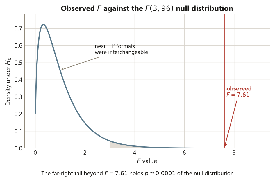
If the four formats truly have equal means, both mean squares estimate the same within-group variance, so \(F\) hovers near \(1\). If the format means genuinely differ, \(\mathrm{MS}_{\text{between}}\) inflates while \(\mathrm{MSE}\) does not, and \(F\) grows. A large \(F\) — far out in the right tail of the \(F(k-1, N-k)\) distribution — is the evidence that some means differ.

Figure 1: Signal over noise — what the \(F\)-ratio compares. Each format’s \(25\) synthetic final scores scatter around its own group mean (the black bar): Lecture \(74\), Lecture+Lab \(81\), Online \(70\), Hybrid \(79\). How far those four bars sit from the dashed grand mean \(76\) is the between-group signal (\(\mathrm{SS}_{\text{between}} = 1850\) on \(3\) df); how widely the dots spread within each column is the within-group noise (\(\mathrm{MSE} = 81\) on \(96\) df). The \(F\)-ratio \(616.7/81 \approx 7.61\) is exactly signal variance over noise variance. Synthetic; seed 35203.

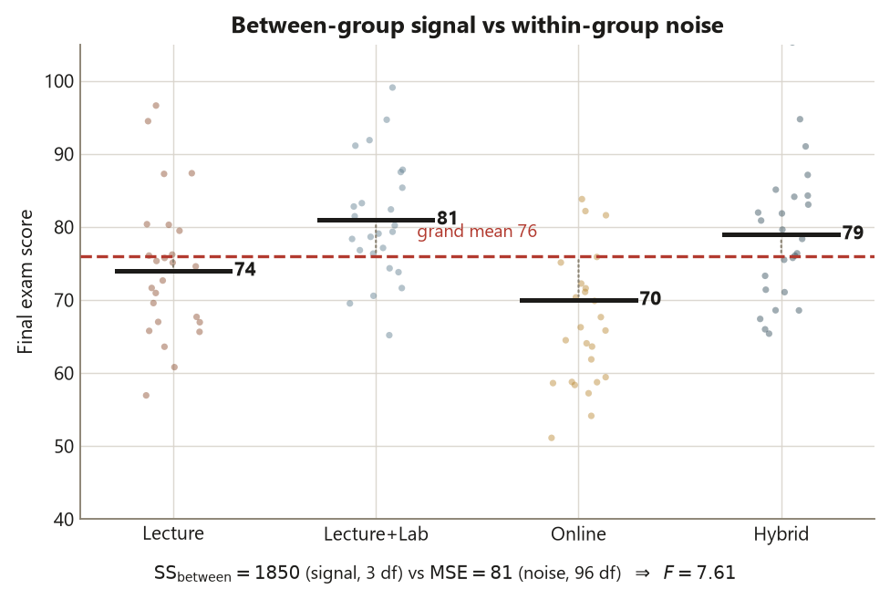
Build it from the locked Dataset F numbers. The four format means are \(L = 74\), \(LL = 81\), \(O = 70\), \(H = 79\), with grand mean \(\bar{\bar x} = 76\) and \(n = 25\) per group (\(N = 100\), \(k = 4\)). The between-group sum of squares weights each squared mean-gap by its group size:

\[ \mathrm{SS}_{\text{between}} = 25\big[(74-76)^2 + (81-76)^2 + (70-76)^2 + (79-76)^2\big] = 25(4 + 25 + 36 + 9) = 1850 , \]

on \(k - 1 = 3\) df, so \(\mathrm{MS}_{\text{between}} = 1850/3 \approx 616.7\). The within-group piece comes from the common within-format SD of about \(9\) points (variance \(81\)): with \(N - k = 96\) residual df, \(\mathrm{SS}_{\text{within}} = 96 \times 81 = 7776\) and \(\mathrm{MSE} = 81\). The ratio is

\[ F = \frac{616.7}{81} \approx 7.61 \quad \text{on } (3, 96)\ \text{df}, \qquad p \approx 0.0001 . \]

An \(F\) of \(7.61\) is well into the right tail of the \(F(3,96)\) distribution — far larger than the value near \(1\) you would expect if the formats were interchangeable — so the omnibus test rejects the null of four equal means. The estimate here is not the \(p\)-value; the \(p\)-value is the verdict. The estimate of how much comes next.

Figure 2: The observed \(F\) sits far out in the null distribution’s tail. The curve is the \(F(3,96)\) sampling distribution the omnibus test would follow if all four format means were equal — it piles up near \(1\). The observed \(F = 7.61\) (red line) lands far to the right, in a region the null almost never reaches: the shaded tail beyond it holds only about \(p \approx 0.0001\) of the distribution. That tiny tail share is why the test rejects “four equal means.” The picture is a statement about surprise under the null, not a measure of how large the format effect is. Synthetic; seed 35203.

eta-squared as the effect size: what a significant F does and does not tell you

A small \(p\) says “some difference exists.” It is silent on how big. For that you report the effect size \(\eta^2\), the share of total score variation the factor explains:

\[ \eta^2 = \frac{\mathrm{SS}_{\text{between}}}{\mathrm{SS}_{\text{total}}} = \frac{\mathrm{SS}_{\text{between}}}{\mathrm{SS}_{\text{between}} + \mathrm{SS}_{\text{within}}} = \frac{1850}{1850 + 7776} = \frac{1850}{9626} \approx 0.19 . \]

So format explains about \(19\%\) of the variance in final scores; the remaining \(81\%\) is student-to-student variation within formats. That single sentence is the estimate-with-its-context that the course demands — never report \(F \approx 7.61\), \(p \approx 0.0001\) and stop, because a bare significant \(p\) can mask a trivial effect when \(N\) is large, or hide a large effect that simply missed the cutoff when \(N\) is small. Naming \(\eta^2 \approx 0.19\) tells a reader the format effect is substantively non-trivial, not just detectable. (You can report \(\eta^2\) with an interval too; here we quote the point value.)

Now the bright line. A significant \(F\) tells you some format means differ. It does not tell you which — not L versus O, not LL versus H, none of the six pairs by itself. Reading “which” off the omnibus \(F\) is exactly the error this week warns against, and answering “which” honestly — with the family-wise rate still controlled — is week 8 (Tukey HSD and planned contrasts). And the conclusion carries one more boundary: because students were not randomly assigned to formats, this is an observational comparison. A real format effect is plausible, but motivated or better-prepared students may have self-selected into Lecture+Lab or Hybrid, so the honest reading is association, not causation — format is associated with a \(\approx 19\%\) share of score variance; the design does not license “format caused the difference.” Week 11 returns to this dataset with a pretest covariate to push on exactly that confound.

Worked examples

Worked example — Dataset F: one-way ANOVA across four formats (recurring slice)

The question and structure. Do the four instructional formats differ in mean final score? The response is final exam score (quantitative); the factor is format with four levels (L, LL, O, H); \(n = 25\) per format, \(N = 100\); the design is observational (no random assignment to format). One quantitative response, one factor with \(> 2\) levels — the structure calls for one-way ANOVA. Data are synthetic; seed set.

The assumptions. ANOVA assumes the within-group residuals are roughly normal, the groups share a common variance (so a single pooled \(\mathrm{MSE}\) is meaningful), and the observations are independent. Here independence holds (different students), the within-format SD is about \(9\) in every group, and the residuals are near-normal with one mild low outlier — an Online student near \(45\). You note that outlier and investigate it; you do not silently delete it. The full diagnostic check — the QQ plot and Levene’s test — is week 7’s business; this week you flag the assumptions and proceed.

The computation. Assemble the ANOVA table from the locked means and SDs:

Source	SS	df	MS	\(F\)	\(p\)
Between (Format)	\(1850\)	\(3\)	\(616.7\)	\(7.61\)	\(\approx 0.0001\)
Within (Residual)	\(7776\)	\(96\)	\(81\)
Total	\(9626\)	\(99\)

The static R below shows the idiom an analyst would run; it is teaching code and is not executed on this site. The key output is shown as a comment.

set.seed(35203)

# Dataset F: final exam score by instructional format. Synthetic.
# 25 students per format (L, LL, O, H); N = 100. Within-format SD ~ 9.
# Group means (locked): L = 74, LL = 81, O = 70, H = 79; grand mean = 76.
final  <- c(L_scores, LL_scores, O_scores, H_scores)   # 100 final scores (response)
format <- factor(rep(c("L", "LL", "O", "H"), each = 25))

fit <- aov(final ~ format)                              # one-way ANOVA: one factor
summary(fit)

#               Df  Sum Sq  Mean Sq  F value   Pr(>F)
# format         3    1850    616.7     7.61   ~1e-04   ***
# Residuals     96    7776     81.0
# ---
# Total SS = 1850 + 7776 = 9626

# Effect size: proportion of score variance explained by format.
eta_sq <- 1850 / 9626                                   # -> ~0.19

The estimate with its uncertainty. The omnibus \(F = 7.61\) on \((3, 96)\) df gives \(p \approx 0.0001\), so you reject the null that all four format means are equal. Reported as an estimate, not just a verdict: format explains \(\eta^2 = 1850/9626 \approx 0.19\) — about \(19\%\) — of the variation in final scores. The means themselves (\(74\), \(81\), \(70\), \(79\)) describe the direction; LL and H sit highest, O lowest, with a \(\approx 11\)-point spread between the extreme group means.

Figure 3: The four format means, each with its 95% confidence interval. Lecture+Lab (\(81\)) and Hybrid (\(79\)) sit above the dashed grand mean of \(76\); Online (\(70\)) sits below, with Lecture (\(74\)) between. Each interval is the mean \(\pm 3.6\) points (standard error \(1.8\) with \(n = 25\) per group), so the \(11\)-point spread from Online to Lecture+Lab is comfortably larger than the intervals — the picture behind the significant omnibus \(F\). The plot shows that the formats differ and by roughly how much; it does not say which specific pairs are distinguishable. Synthetic; seed 35203.

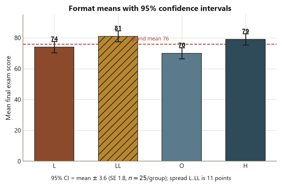
The interpretation. Some formats differ in mean final score, and the difference is substantively non-trivial (a \(\approx 19\%\) variance share, not a sliver). But two boundaries hold firmly. First, the \(F\) does not identify which formats differ — O looks lowest and LL highest, yet which specific pairs are distinguishable, with the family-wise error controlled, is week 8, not something to read off the omnibus result. Second, the design is observational: students self-selected formats, so this is association, not causation — you cannot conclude that switching a student to Lecture+Lab would raise their score; you can only say format is associated with score here. That is the whole blueprint walked once: question, structure, method, assumptions, an estimate with its uncertainty, and a conclusion that states what it cannot support.

Worked example — three fertilizers and crop yield (transfer, new context)

The question and structure. An agronomy station compares crop yield (bushels per plot) under three fertilizer formulations — call them A, B, and C — applied to \(30\) plots each, \(N = 90\). The response is yield (quantitative); the factor is fertilizer with three levels; the plots were randomly assigned to formulations (an experiment, unlike Dataset F). One quantitative response, one three-level factor — again one-way ANOVA. These numbers are illustrative and deliberately distinct from Dataset F.

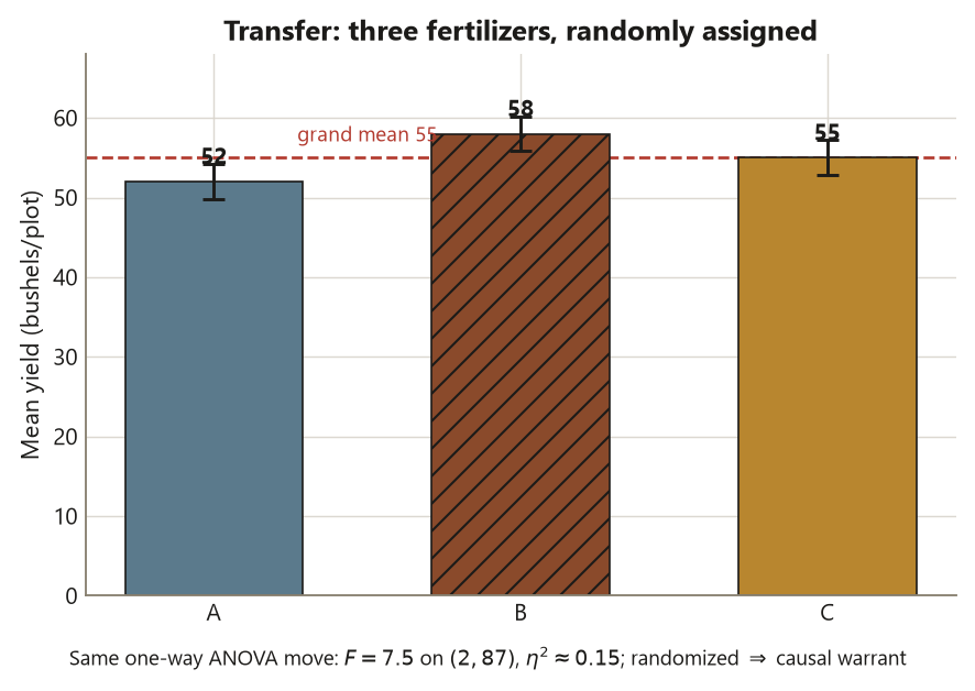
The assumptions and the F-ratio logic. Suppose the three plot-mean yields are \(\bar x_A = 52\), \(\bar x_B = 58\), \(\bar x_C = 55\), grand mean \(\bar{\bar x} = 55\), with a common within-group SD of about \(6\) (so \(\mathrm{MSE} = 36\)) and \(n = 30\) per group. The same machinery applies. Between-group:

\[ \mathrm{SS}_{\text{between}} = 30\big[(52-55)^2 + (58-55)^2 + (55-55)^2\big] = 30(9 + 9 + 0) = 540 , \]

on \(k - 1 = 2\) df, so \(\mathrm{MS}_{\text{between}} = 270\). Within-group: \(\mathrm{SS}_{\text{within}} = (N-k)\,\mathrm{MSE} = 87 \times 36 = 3132\) on \(87\) df, with \(\mathrm{MSE} = 36\). The ratio is

\[ F = \frac{\mathrm{MS}_{\text{between}}}{\mathrm{MSE}} = \frac{270}{36} = 7.5 \quad \text{on } (2, 87)\ \text{df}, \]

an \(F\) well above \(1\), so the omnibus test would flag that some fertilizer mean differs. The effect size is \(\eta^2 = 540/(540 + 3132) = 540/3672 \approx 0.15\) — fertilizer explains about \(15\%\) of yield variance.

Figure 4: The same design move in a new context. Three fertilizer formulations give mean yields of \(A = 52\), \(B = 58\), \(C = 55\) bushels per plot around a grand mean of \(55\), each with a \(95\%\) interval of about \(\pm 2.2\) (standard error \(1.1\), \(n = 30\) per plot-group). The one-way ANOVA machinery is identical to Dataset F — signal between the group means over noise within them, \(F = 7.5\) on \((2, 87)\), \(\eta^2 \approx 0.15\) — only the units and numbers change. What does change is the warrant: the plots were randomly assigned, so a real difference here can support a causal reading, unlike the self-selected formats. Synthetic; illustrative, distinct from Dataset F.

set.seed(35203)

# Fertilizer trial (transfer): yield (bushels/plot) under 3 formulations.
# Synthetic, illustrative; 30 plots per fertilizer, N = 90, within-group SD ~ 6.
# Means: A = 52, B = 58, C = 55; grand mean = 55.
yield      <- c(A_yield, B_yield, C_yield)             # 90 plot yields (response)
fertilizer <- factor(rep(c("A", "B", "C"), each = 30))

fit2 <- aov(yield ~ fertilizer)
summary(fit2)

#               Df  Sum Sq  Mean Sq  F value
# fertilizer     2     540    270.0     7.50
# Residuals     87    3132     36.0

eta_sq2 <- 540 / 3672                                   # -> ~0.15

The interpretation — and one design contrast worth naming. The omnibus \(F = 7.5\) on \((2, 87)\) df says some fertilizer mean differs, and \(\eta^2 \approx 0.15\) estimates how much. The structure is identical to Dataset F — one quantitative response, one factor, the same signal-over-noise \(F\) — so only the context and the numbers changed. But one thing did change that the conclusion must honor: here the plots were randomly assigned to fertilizers, so a significant difference can support a causal reading (fertilizer affects yield), whereas Dataset F’s self-selected formats bought only association. Same method, same \(F\)-logic, different causal warrant — set by the design, exactly as the blueprint insists. And as always, the \(F\) alone does not say which fertilizer wins; that comparison, with the family-wise rate controlled, is the next layer.

A common mistake

This week’s classic error has three faces, and all three trade an honest estimate for an overstated verdict (Risk 1, Risk 6 in the convention list).

The first and worst is running unadjusted pairwise \(t\)-tests instead of — or carelessly after — the ANOVA, with no error-rate control. With four formats that is six tests, and at the \(5\%\) level the family-wise false-alarm rate climbs toward \(26\%\), not \(5\%\). The fix is the omnibus ANOVA first, then a multiplicity-controlled procedure (Tukey HSD, Bonferroni, or a planned contrast) for the pairwise question — week 8. Reaching straight for six bare \(t\)-tests means your “significant” pairs are running at an advertised rate you never actually held. Run the omnibus gate first; control the family rate before you trust any pair.

Figure 5: Why six unadjusted tests is not a \(5\%\) procedure. Each added pairwise \(t\)-test at the \(5\%\) level is another chance for a false alarm, so the probability that at least one of them fires by luck — even when every format is truly identical — climbs as \(1 - 0.95^{m}\). By the \(m = 6\) comparisons among four formats it has already reached about \(0.26\) (red point), five times the \(0.05\) you advertised (dashed line). Running the omnibus ANOVA first, then a multiplicity-controlled follow-up, is what keeps the family-wise rate at the level you claimed. Synthetic; illustrative.

The second is reporting \(F\) with no effect size — writing “\(F = 7.61\), \(p \approx 0.0001\), significant” and stopping. That is a bare verdict, and this course never accepts a bare verdict. A significant \(F\) with a large \(N\) can accompany a trivially small effect; a real effect can miss the cutoff in a small study. Always pair the test with \(\eta^2\) (here \(\approx 0.19\)) so a reader knows how much of the response the factor explains, not merely that something is detectable. Estimate with its uncertainty, never a lone p-value.

The third is concluding which groups differ from the omnibus \(F\) alone — reading “\(O\) is lowest, so \(O\) differs from \(LL\)” straight off the significant ANOVA. The omnibus \(F\) answers only “do any differ?” It cannot single out a pair; the four means and one \(F\) do not contain a multiplicity-controlled pairwise verdict. Pointing at the biggest gap and declaring it significant re-imports the very family-wise inflation ANOVA was run to avoid. Say “some formats differ (\(\eta^2 \approx 0.19\)); which pairs differ, with the error rate controlled, is the next step,” and leave the “which” to week 8.

Low-stakes self-checks (ungraded)

These are for your own practice — ungraded, no submission.

1. In one sentence, explain why running all six pairwise \(t\)-tests among four formats at the \(5\%\) level does not give you an overall \(5\%\) error rate, using the phrase family-wise error.
2. For Dataset F, identify the response, the factor and its levels, the unit of analysis, and the design (observational or experimental). Which of these decides that the conclusion is association, not causation?
3. Reproduce the between-group sum of squares from the means: show that \(25[(74-76)^2 + (81-76)^2 + (70-76)^2 + (79-76)^2] = 1850\), and state its degrees of freedom.
4. The ANOVA gives \(F \approx 7.61\) and \(\eta^2 \approx 0.19\). Write one sentence reporting the result as an estimate with its meaning (not a bare p-value), and one sentence saying what the \(F\) does not tell you about individual format pairs.
5. A classmate writes: “The ANOVA was significant, so Online is significantly worse than Lecture+Lab.” Name the error and the correct scope of what the omnibus \(F\) supports.
6. In the fertilizer transfer example the plots were randomly assigned, but in Dataset F students self-selected their format. Explain in one sentence how that single difference changes the conclusion you may draw from the same significant \(F\).

Reading and source pointer

This week is grounded in the instructor notes (the primary course materials) for the one-way ANOVA framing — the omnibus-test logic, the partition of variance into between and within, and the insistence on \(\eta^2\) as the reported effect size — alongside the IMS (Çetinkaya-Rundel & Hardin) treatment of comparing many means (ANOVA) for the concept sequence (the \(F\)-ratio and the variance partition), and the ModernDive (Ismay, Kim & Valdivia) treatment of modeling with a categorical predictor for the R workflow that fits the model and reads the output table. These notes are the course’s own synthesis, grounded in but not copied from the sources. No prose, examples, exercises, figures, or solutions are reproduced from any source.

Public vs. graded

These notes, the examples, and the practice here are public and ungraded — study material only. No graded prompts, answer keys, rubrics, point values, or due dates appear on this site. Graded applied-methods checkpoints, weekly quizzes, homework and analysis memos, applied analysis labs, the midterm, the applied methods project, and the final exam live in Blackboard (the LMS), which is authoritative for due dates, submissions, and grades. If this page and Blackboard ever disagree, follow Blackboard.

Looking ahead

Next week we stop assuming the ANOVA’s assumptions and start checking them: the residual QQ plot for near-normality, Levene’s test for equal variances (Dataset F gives \(p \approx 0.40\), so equal-variance is reasonable), and what to do with that one mild Online outlier near \(45\) — investigate, do not auto-delete. That diagnostics work also consolidates the first arc of the course — applied workflow, exploratory analysis, estimation and uncertainty, paired and two-group comparisons, and this week’s one-way ANOVA — into one habit of checking before you trust. The omnibus gate you built here is only as honest as the assumptions underneath it, so checking them is the natural next move before you ever ask which groups differ.

See also

• Week 5 — Two-group comparisons — the two-group case this week generalizes; why four groups is not “just six of those.”
• Week 7 — Assumptions, diagnostics & the midterm — checking the normality, equal-variance, and independence assumptions ANOVA rests on.
• Week 8 — Multiple comparisons & planned contrasts — the “which groups differ?” question, with the family-wise error rate controlled.
• Assumptions and diagnostics guide — the residual, variance, and independence checks in one place.
• Method chooser — the question → structure → method decision guide that routes “one quantitative response, one factor, several levels” to one-way ANOVA.