Week 1 — Statistical questions, data structure & applied workflow

From a question to variables, a method, an estimate, and a bounded conclusion

The week question

This course is not a tour of named tests. It is one habit, practiced on many kinds of data, until the habit becomes automatic. The habit is to refuse to reach for a method until you have said, out loud and in order, what you are asking and what your data actually look like. So the question for week 1 is the question that sits underneath every other week: given a real applied question and a real data table, how do you move — deliberately and in the right order — from the question to the variables, to a method that matches the structure, to an estimate reported with its uncertainty, and to a conclusion that does not claim more than the data can support?

That ordered move is the course’s spine. We will call it the analysis blueprint, and it has six steps: Question, Structure, Method, Assumptions, Estimate, Conclusion. Every week from here forward — the paired \(t\), the two-sample \(t\), one-way and two-way ANOVA, ANCOVA, regression, the chi-square test, logistic regression — is the same six steps walked across a different data structure. If you learn the blueprint this week, the rest of the course is recognition: you will keep meeting structures you have a move for, rather than a box of tests you have to guess among.

To make that concrete, this week introduces the world we will return to all term — the Cypress Ridge College Student-Success Study — as five datasets of different structures. We will not compute much this week. We will instead learn to read a structure and say which method it is going to call for, so that when each method arrives you already know why it is the right tool for that shape of data.

Why this matters

Most people, asked to analyze data, start at step 3. They have a question in mind, glance at the spreadsheet, and immediately reach for a test they remember — “let’s do a \(t\)-test,” “let’s run a regression.” That instinct is exactly backwards, and it is the single most expensive error in applied work, because a method chosen before the structure is understood is often the wrong method, quietly producing a number that looks authoritative and means something other than you think.

Consider one concrete trap you will see all term. Dataset P measures the same 30 students before and after a support module; Dataset G measures different students in two groups. Both compare two sets of scores. But P is paired and G is independent, and that single structural fact — same units or different units — changes which standard error you compute, which test you run, and how much power you have. Get the structure right and the method follows almost mechanically. Get it wrong and a paired study analyzed as two independent samples throws away its best feature: that each student is their own control.

There is a second, quieter reason this matters, and it runs through every page of this course. A method does not just hand you a verdict; it hands you an estimate — a mean difference, a slope, an odds ratio — and that estimate comes with uncertainty. The discipline of this course is to report the estimate with its uncertainty, never a bare p-value, and to keep three things separate that students constantly collapse: statistical significance (could this be noise?), practical significance (is the effect big enough to matter?), and causation (did the explanatory variable cause the change, or merely travel with it?). Observational data — and several of our datasets are observational — buy you association, not causation. Naming that boundary honestly is part of the analysis, not an afterthought.

So the blueprint is not bureaucracy. It is the difference between an analysis you can defend and a number you merely produced.

Learning goals

By the end of this week you should be able to:

• State the six-step analysis blueprint — Question, Structure, Method, Assumptions, Estimate, Conclusion — and explain why structure (step 2) must precede method (step 3).
• Read a data table and identify its structure: the unit of analysis; which variable is the response versus an explanatory variable, a grouping factor, or a covariate; the outcome type (quantitative, categorical, or binary); and the design (paired vs independent, one factor vs two, observational vs experimental).
• Walk each of the five Cypress Ridge datasets through blueprint steps 1–3 and name which method its structure calls for — and say why that one and not a neighbor.
• Explain, in plain words, the two disciplines that recur on every page: report the estimate with its uncertainty, not a bare verdict, and keep statistical significance, practical significance, and causation distinct.
• Take a brand-new applied question in an unfamiliar context and complete steps 1–2 — unit, response, explanatory variable, outcome type, design — before naming any test.

Core vocabulary

• Analysis blueprint — the six ordered steps the course applies to every method: (1) Question (comparing, explaining, or predicting?), (2) Structure (units and variables and design), (3) Method (the analysis matching that structure), (4) Assumptions & diagnostics, (5) Estimate & uncertainty, (6) Conclusion. A method is one instance of this blueprint, not a freestanding test.
• Unit of analysis — the thing a row of the data table represents and on which the response is measured: a student, a class, a seed, a clinic visit. Get this wrong and everything downstream tilts.
• Response variable (\(Y\)) — the outcome you want to compare, explain, or predict (a final score, a pass/fail flag, a wait time).
• Explanatory variable / grouping factor / covariate — variables that might account for the response. A grouping factor is categorical and sorts units into groups (format, program); an explanatory variable can be quantitative (study hours); a covariate is a quantitative variable you adjust for rather than focus on (a baseline pretest).
• Outcome type — whether the response is quantitative (a number, like a 0–100 score), categorical/nominal (an unordered class), or binary (two outcomes, like pass/fail). The type steers the method: quantitative responses point toward \(t\)-tests, ANOVA, and regression; binary responses point toward chi-square and logistic regression.
• Design — how the data were produced: paired vs independent (same units measured twice, or different units?); one factor vs two (one grouping variable, or a crossing of two?); observational vs experimental (did the analyst assign the conditions, or merely observe them?). Design decides both the method and what the conclusion is allowed to say.
• Estimate with uncertainty — the model’s answer reported as a point estimate plus a confidence interval (and an effect size), never as a lone p-value.
• Statistical vs practical significance; association vs causation — the three claims to keep apart: is it more than noise; is it big enough to matter; and did \(X\) cause the change or merely accompany it?

Concept development

What a statistical question is, and the six-step blueprint

A statistical question is one whose answer depends on variation in data and that can be settled, at least partly, by an estimate computed from that data. “Did this student improve?” is not statistical — it is one number. “Does the support module improve readiness on average, and by how much, beyond what we’d see by chance?” is statistical: it asks about a population, expects an estimate, and admits uncertainty.

Notice that a good statistical question already commits you to a verb. You are almost always doing one of three things:

• Comparing — is the response different across groups or conditions? (formats, programs, support vs self-guided.)
• Explaining / adjusting — how does the response change with an explanatory variable, holding other things fixed? (final score as study hours rise, adjusting for attendance and a pretest.)
• Predicting — given inputs, what outcome do we expect? (the probability a student passes.)

The verb is step 1 of the blueprint. The blueprint then continues, and the order is not negotiable:

1. Question — comparing, explaining, or predicting?
2. Structure — unit of analysis; response vs explanatory / grouping / covariate; outcome type; design.
3. Method — the analysis whose assumptions and inputs match that structure.
4. Assumptions & diagnostics — what the method assumes, and how you check it.
5. Estimate & uncertainty — what the model estimates (a mean difference, a slope, an odds ratio), reported with a confidence interval, never as a bare p-value.
6. Conclusion — statistical vs practical significance; association vs causation; what the analysis can and cannot support.

Figure 1: The analysis blueprint: six ordered steps, walked on every method. Every method this term — the paired \(t\), the two-sample \(t\), one-way and two-way ANOVA, ANCOVA, regression, chi-square, logistic regression — is these same six steps applied to a different data structure. Step 2 (Structure, highlighted) is the load-bearing one: the shape of the data names the method in step 3, which is why you read the structure before you reach for a test. The blueprint is the course’s spine, meant to become automatic, not a checklist to memorize.

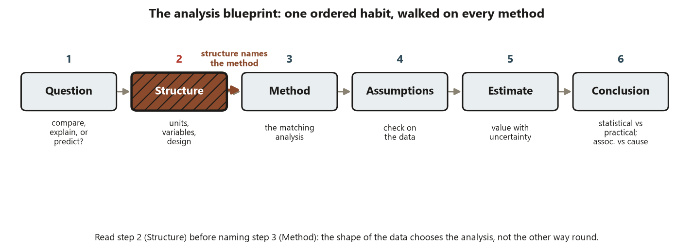
The load-bearing claim of the whole course is that step 2 determines step 3. You do not pick a method and then bend the data to fit; you read the structure and let it name the method. That is why this week spends its energy on reading structures rather than running tests.

Data structure: units, variable roles, outcome type, and design

Structure has four readable parts, and you should train yourself to answer all four before going further.

Unit of analysis. Look at one row of the table. What does it stand for? In Dataset P each row is a student, carrying that student’s pre and post score. In Dataset F each row is a student in one of four instructional formats. The unit matters because the response is measured per unit, and the design (paired or not) is a statement about whether the same units recur.

Variable roles. Sort the columns. The response \(Y\) is what you want to learn about. The rest are candidate explanations: a grouping factor (categorical — format, program, delivery), an explanatory variable (often quantitative — study hours), or a covariate you will adjust for rather than feature (a baseline pretest). The same column can play different roles in different questions — a pretest is the response in week 4’s paired study but a covariate in week 11’s ANCOVA — so the role is something you assign relative to the question, not a fixed property of the column.

Outcome type. Is \(Y\) quantitative, categorical, or binary? A 0–100 final score is quantitative and opens the door to means, \(t\)-tests, ANOVA, and regression. A pass/fail flag is binary and points instead toward proportions, contingency tables, and logistic regression. Type is the first fork in the road: you cannot run a \(t\)-test on a pass/fail outcome, and you would not run a chi-square on a continuous score.

Design. Three questions. Paired or independent? — are two measurements on the same units (paired, like P’s pre/post) or on different units (independent, like G’s two groups)? One factor or two? — is there a single grouping variable (F’s one Format factor) or a crossing of two (X’s Delivery \(\times\) Background)? Observational or experimental? — did the analyst assign the condition, or merely record it? G and the program comparison in R are observational — students self-selected — which is exactly why their conclusions will be capped at association, not causation.

The applied workflow, and the four “not this” boundaries

Putting it together, the applied workflow this course teaches is: read the question, read the structure, let the structure name the method, check the method’s assumptions on the actual data, estimate the quantity of interest with its uncertainty, and conclude with the three claims kept distinct. R and Quarto carry out the fit and print the output; they are the hands, not the head.

That workflow is defined as much by what it refuses to be. Resist all four drifts:

• Not generic intro statistics. Descriptive summaries, the normal model, a single one-sample \(t\), the bare mechanics of one confidence interval — these are assumed background. Our subject is choosing and connecting a method to a structure across groups, factors, covariates, and categorical outcomes.
• Not a pure R / software course. Code runs the analysis; the method’s logic — what is compared, assumed, estimated, concluded — is the message. We will read code, but the code is never the point.
• Not a formula-only methods course. The goal is never to memorize a test statistic or its sampling distribution. It is to map question → structure → method → estimate → conclusion and to read real output.
• Not a disconnected catalog of named tests. The paired \(t\), two-sample \(t\), ANOVA, two-way ANOVA, ANCOVA, regression, chi-square, and logistic regression are not a box of “use this when…”. They are connected expressions of one blueprint. A method is a way to connect a question, a structure, an estimate, an uncertainty, and a conclusion — not an item on a menu.

Hold that last sentence. It is the thesis of the course, and the five datasets exist to demonstrate it.

Worked examples

Worked example — the five Cypress Ridge structures through blueprint steps 1–3 (recurring slice)

What is assumed. All five datasets are slices of one synthetic world — the Cypress Ridge College Student-Success Study, a redesign of a quantitative-reasoning course and its tutoring/support program. Data are synthetic; seed set with set.seed(35203); they are not real records. There are no load-bearing statistics this week — the only thing we lock is each dataset’s structure and the method it will call for. We are practicing steps 1–3 only: name the question, read the structure, name the method.

Figure 2: One study, five structures. The Cypress Ridge world arrives as five datasets whose shapes differ, and it is the shape — not the topic — that calls for each method. P is paired: the same \(n = 30\) students measured twice (pre linked to post). G is two independent groups (\(45 + 45\) different students). F is one factor with four formats (\(n = 25\) each). X crosses two factors in a \(2\times2\) design (\(n = 20\) per cell). R relates a quantitative predictor to an outcome (\(n = 120\)). Read the shape first; the method follows. Synthetic; seed 35203.

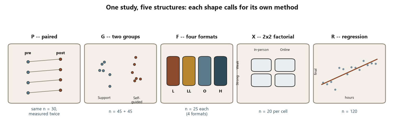
Walk each dataset:

• P — paired pre/post readiness. Question: did readiness change after the support module (comparing)? Structure: unit = student; the same \(n = 30\) students measured twice (pre, post); response = readiness score (quantitative); design = paired, one factor (time), observational. Method: the paired \(t\) — because the two measurements share a unit, you analyze each student’s difference and remove between-student variation. (Treating these as two independent samples would be the classic structural error.)
• G — final scores: Support vs Self-guided. Question: do support-center users score differently (comparing)? Structure: unit = student; two independent groups of different students (\(n_1 = 45\) Support, \(n_2 = 45\) Self-guided); response = final score (quantitative); design = independent, one factor, observational (students self-selected). Method: the two-sample \(t\) (Welch by default) — different units, so a between-groups comparison, not a paired one.
• F — final score by instructional Format. Question: do the four formats differ (comparing >2 groups)? Structure: unit = student; one grouping factor with four levels (Lecture, Lecture+Lab, Online, Hybrid), \(n = 25\) each; response = final score (quantitative); design = one factor, observational. Method: one-way ANOVA — comparing more than two group means at once, which is what ANOVA is for.
• X — Delivery \(\times\) Background. Question: does delivery format interact with prior background (comparing across a crossing)? Structure: unit = student; two crossed factors — Delivery {In-person, Online} \(\times\) Background {Weak, Strong}, \(n = 20\) per cell; response = final score (quantitative); design = two factors. Method: two-way ANOVA — two factors at once, and crucially a check for interaction (does the effect of one factor depend on the other?).
• R — hours / attendance / pretest / program → final score & pass/fail. Question: how does final score depend on study hours and other inputs (explaining/predicting), and what drives passing (predicting a binary outcome)? Structure: unit = student (\(n = 120\)); quantitative explanatory variables (hours, attendance, pretest), a grouping factor (program), and two response types — a quantitative final score and a binary pass/fail. Method: regression (simple and multiple) for the quantitative response, a contingency table / chi-square for pass \(\times\) program, and logistic regression for the binary pass outcome.

A compact map is the cleanest way to hold this:

Dataset	Structure (unit · response · design)	Method it calls for
P	same 30 students, measured twice; quantitative; paired	paired \(t\)
G	two independent groups (45 + 45); quantitative; observational	two-sample \(t\) (Welch)
F	one factor, four formats (\(n=25\) each); quantitative	one-way ANOVA
X	two crossed factors (\(2\times2\), \(n=20\)/cell); quantitative	two-way ANOVA (interaction)
R	predictors + program; quantitative and binary responses	regression · chi-square · logistic

Figure 3: Structure names the method. The same map sits behind every week of the course: each data structure on the left (step 2) generates exactly one analysis on the right (step 3). Paired data call for the paired \(t\); two independent groups for the two-sample (Welch) \(t\); one factor with more than two groups for one-way ANOVA; two crossed factors for two-way ANOVA with an interaction check; a quantitative predictor for regression; a categorical or binary outcome for chi-square or logistic regression. The letters P, G, F, X, R tag the five Cypress Ridge datasets, so each row is a week you will meet. Synthetic; seed 35203.

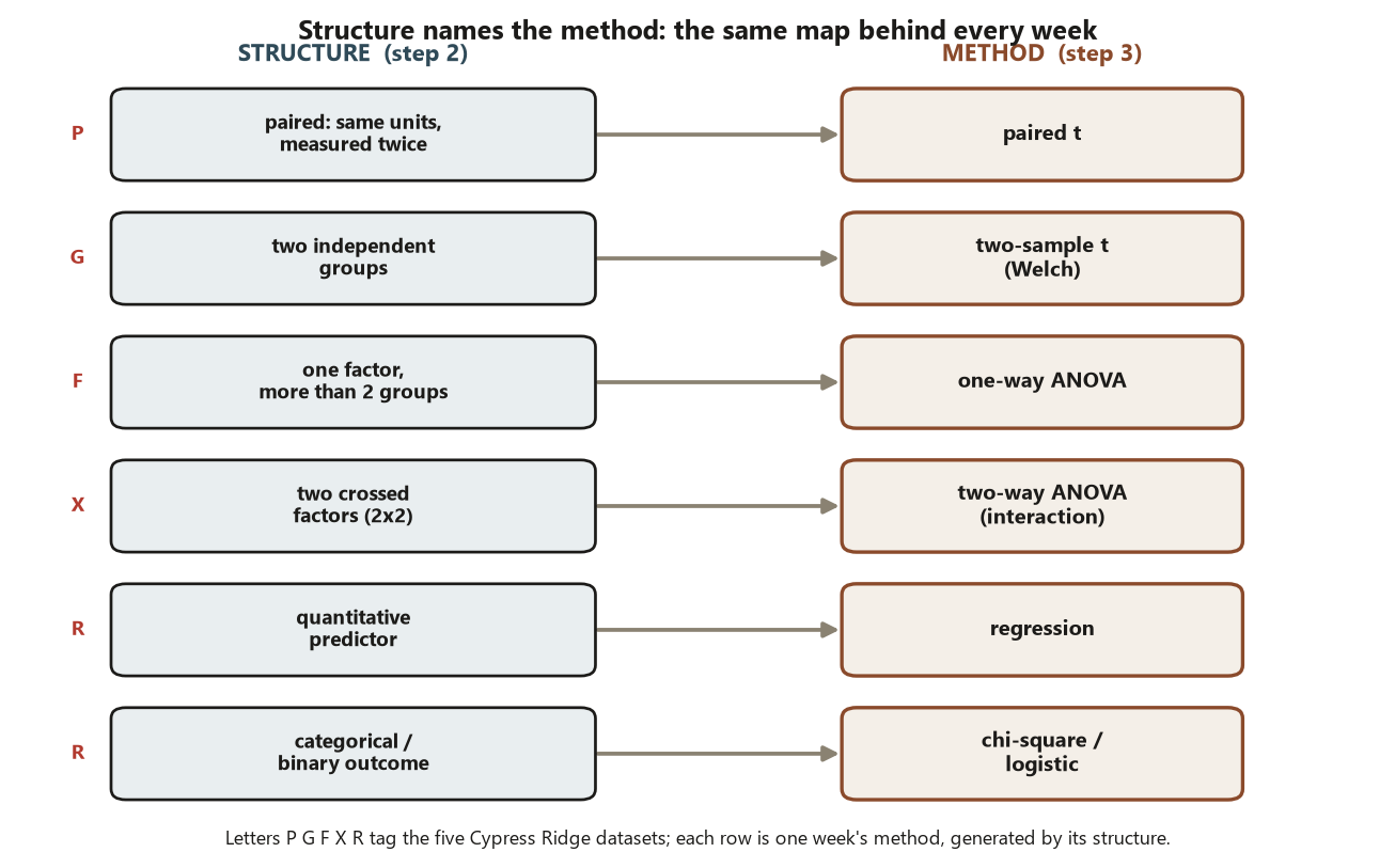
Now make the structure literally visible. The static R below inspects the shape of two of these tables — the kind of look you take before naming any method. It is teaching code and is not executed here.

set.seed(35203)

# Dataset P (paired): one row per student, the SAME student measured twice.
str(readiness_P)
#> 'data.frame': 30 obs. of  3 variables:
#>  $ student: int  1 2 3 4 5 ...
#>  $ pre    : num  58 65 60 71 55 ...   # quantitative response, time 1
#>  $ post   : num  64 70 63 79 61 ...   # quantitative response, time 2
# Two columns ARE the two measurements -> PAIRED structure -> paired t.

# Dataset F (one factor, four groups): one row per student, a Format label.
str(scores_F)
#> 'data.frame': 100 obs. of  2 variables:
#>  $ format: Factor w/ 4 levels "L","LL","O","H": 1 1 1 2 2 ...  # grouping factor
#>  $ final : num  74 71 78 83 80 ...    # quantitative response
table(scores_F$format)
#>  L LL  O  H
#> 25 25 25 25            # one factor, 4 levels, n = 25 each -> one-way ANOVA.

The interpretation. Nothing here is a result — there is no estimate, no p-value, no confidence interval yet. That is the point. The str() and table() output tells you the unit (a student per row), the response type (quantitative scores), the roles (a format grouping factor), and the design (P’s two score columns reveal pairing; F’s four equal-\(n\) levels reveal a single factor). The structure named the method for each dataset before any arithmetic happened. Step 5 (the estimate with its uncertainty) and step 6 (the bounded conclusion) arrive in later weeks; this week we earn the right to those steps by reading structure correctly first.

Worked example — a campus clinic kiosk (transfer, new context)

What is assumed. Step out of the Cypress Ridge world entirely. A campus health clinic installs a new self-service check-in kiosk and asks whether it shortens visit times. These numbers are illustrative and clearly distinct from the five datasets; the exercise is to complete blueprint steps 1–2 before naming any test.

The reading. Take the four structural questions in order.

• Question (step 1). Are we comparing, explaining, or predicting? We are comparing — visit times with the kiosk against visit times without it.
• Unit of analysis. What is one row? A clinic visit (or a patient-visit). The response is measured per visit, so the visit is the unit — not the day, not the clinic.
• Response and its type. The response \(Y\) is visit time in minutes — quantitative. (If the clinic had instead asked “did the visit finish within the target 30 minutes — yes/no?”, the response would be binary, and the whole downstream path would change. Type is a fork in the road.)
• Explanatory variable. The grouping factor is the check-in method: kiosk vs front-desk. It is categorical with two levels.
• Design (the decisive read). Paired or independent? If the clinic compares different visits — some checked in by kiosk, some at the desk — the design is independent (two separate groups of visits), pointing toward a two-sample \(t\), the structure of Dataset G. If instead the same clinic is measured before the kiosk and after its installation, those are two conditions but still different visits, so they are independent unless a single unit is genuinely measured twice. Observational or experimental? — this is the conclusion-capping question. If visits were randomly assigned to kiosk vs desk, a difference can support a causal reading. If patients chose the kiosk (tech-comfortable, perhaps younger patients self-select), the design is observational, and even a clear, statistically significant time difference buys only association — kiosk users might be faster for reasons unrelated to the kiosk.

The interpretation. We have not named a test, and that restraint is the lesson. By finishing steps 1–2 — comparing; unit = visit; response = visit time, quantitative; factor = check-in method, two levels; design = independent and (likely) observational — the method names itself: a two-sample comparison of mean visit times, reported as an estimated mean difference with a confidence interval and an effect size, concluded with statistical-vs-practical significance kept separate and a frank note that self-selected kiosk use means association, not causation. Same six steps, new building, new numbers. That portability is exactly what the blueprint buys you.

A common mistake

This week’s classic applied error is reaching for a named test before identifying the question and the data structure — jumping straight to step 3 and skipping steps 1 and 2. It is so common because it feels efficient: you recognize “two columns of scores” and your hand moves toward “\(t\)-test” before you have asked which \(t\)-test, or whether a \(t\)-test is even right. The blueprint exists to interrupt that reflex.

The mistake takes two recurring shapes. The first is confusing the response and the explanatory roles. If you treat the grouping factor as the outcome — say, trying to “predict format from final score” when the question is whether final score differs by format — you will set up the wrong analysis and answer a question nobody asked. Fix it at step 2: name \(Y\) (the thing you want to learn about, the final score) and the explanatory variables (what might account for it, the format) explicitly, before going on.

The second shape is missing that a design is paired. Dataset P’s pre and post scores are two columns that look like any two columns of numbers; a student who skips step 2 sees “two sets of scores” and runs a two-sample \(t\) as if they were independent groups. But the rows are the same 30 students measured twice. Analyzing P as independent throws away the pairing — and pairing is its whole advantage, because each student serves as their own control and between-student variation is removed. The structural tell is the unit: if one row carries both numbers for one student, the measurements are paired. Read the unit, and the design announces itself.

Figure 4: One reflex, two structures — only one of them fits. “Two columns of scores” tempts the reflex to just run a two-sample \(t\) (top). That is correct for Dataset G, where the two columns are different, independent students. But it is wrong for Dataset P, whose two columns are the same 30 students measured twice: applied to P, the two-sample \(t\) ignores the pairing, and the standard error nearly doubles (the paired analysis is the more powerful one). The two designs look identical on the page; only reading the structure at step 2 tells them apart. Synthetic; seed 35203.

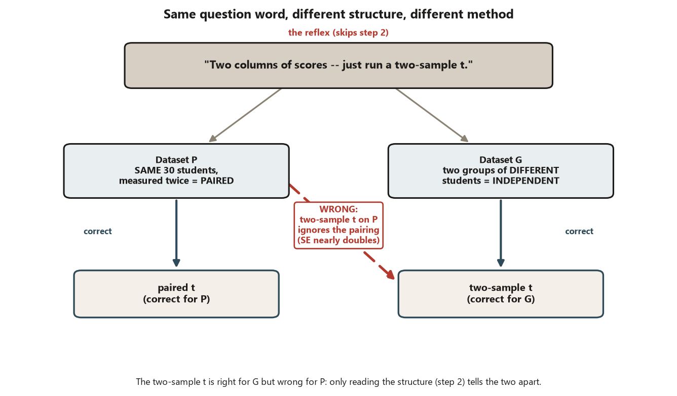
Both shapes have the same cure and the same diagnostic. The cure: never let your hand reach step 3 before your head has finished step 2. The diagnostic: if you cannot state, in one sentence each, the unit of analysis, which variable is the response, and whether the design is paired or independent, observational or experimental — then you are not ready to name a method, and any method you name is a guess.

Low-stakes self-checks (ungraded)

These are for your own practice — ungraded, no submission.

1. In one sentence, state the six steps of the analysis blueprint in order, and say why step 2 (structure) must come before step 3 (method).
2. For Dataset P, name the unit of analysis, the response and its type, and the design (paired or independent; observational or experimental). Then name the method its structure calls for.
3. Datasets P and G both “compare two sets of scores.” In two sentences, explain the structural difference between them and why it leads to different methods.
4. A classmate says, “It’s two columns of numbers, so it’s a two-sample \(t\)-test.” Name the blueprint step they skipped, and describe one dataset above where that conclusion would be wrong.
5. For the campus-clinic kiosk question, write the response variable and its type, the grouping factor, and one feature of the design that would decide whether the conclusion can be causal or only associational.
6. Pick any two of the five datasets and, in one sentence each, name the method its structure calls for and the reason — “why this one and not a neighbor.”

Reading and source pointer

This week is grounded in the instructor notes (the primary course materials) for the analysis blueprint, the applied workflow, and the five-dataset Cypress Ridge world, with the IMS (Cetinkaya-Rundel & Hardin) treatment of data basics and the introduction to exploratory analysis for the vocabulary of variables and data structure — units of observation, response versus explanatory variables, and variable types (numerical vs categorical). IMS grounds the concepts and terminology for reading a data table; the blueprint and the dataset world are the course’s own architecture. These notes are the course’s own synthesis, grounded in but not copied from the sources. No prose, examples, exercises, figures, or solutions are reproduced from any source.

Public vs. graded

These notes, the examples, and the practice here are public and ungraded — study material only. No graded prompts, answer keys, rubrics, point values, or due dates appear on this site. Graded applied-methods checkpoints, weekly quizzes, homework and analysis memos, applied analysis labs, the midterm, the applied methods project, and the final exam live in Blackboard (the LMS), which is authoritative for due dates, submissions, and grades. If this page and Blackboard ever disagree, follow Blackboard.

Looking ahead

Next week we look at the data before fitting anything. Having read a structure on paper, you will put it on a graph: side-by-side boxplots of final score by format (Dataset F) and a scatterplot of study hours against final score (Dataset R), with the numerical summaries that go with them. The point of week 2 is that you should see the comparison or the relationship in a picture before you estimate it — the graph checks whether the structure you read actually behaves the way the method you are about to choose assumes. Exploratory analysis is step 2 made visible, and it is the bridge to every estimate that follows.

See also

• Method chooser — the question → structure → method decision guide, the blueprint’s steps 1–3 as a single chart.
• Methods glossary — unit of analysis, response vs explanatory, outcome type, design, estimate-with-uncertainty.
• Week 2 — Exploratory analysis & graphical comparison — seeing the structure in a graph before fitting anything.
• Week 5 — Two-group comparisons — Dataset G’s independent structure becomes the two-sample \(t\), the first full walk through all six blueprint steps.