Week 4 — One-sample & paired comparisons

When each unit is its own control: differences, not groups

The week question

Last week you took a six-point gap between two groups of students and reported it the responsible way — as a point estimate carried with its confidence interval and an effect size, not as a bare verdict. Those were two different groups of students, though, and the gap was a comparison across units. This week the structure changes in a way that is easy to miss and easy to get wrong. You measure the same thirty students twice — a readiness diagnostic before a six-week support module and the same diagnostic after it — and you ask whether they improved. The question sounds identical to a two-group question, but it is not, because the design is not the same. Each student is paired with themselves, and that pairing is the whole story.

So the week’s question is really two questions stacked. First: how do you do inference on a single mean — a point estimate, a standard error, a confidence interval — as the base case the rest of the course builds on? And second, the one that defines the week: when each unit is measured twice, what exactly do you analyze? The answer is the load-bearing move of the week. You do not compare two clouds of numbers. You collapse each student’s two readings into a single difference, and then you run a one-sample analysis on those thirty differences. The pairing is not a complication to work around; it is the feature that makes the analysis sharper. Same blueprint as always — question, structure, method, assumptions, estimate with uncertainty, conclusion — but here step 2, the structure, is the step that quietly decides everything else.

Why this matters

The reason this matters is not that the paired \(t\)-test is a hard formula. It is not — it is just a one-sample \(t\)-test wearing a costume. The reason it matters is that the design dictates the method, and a reader who skips step 2 of the blueprint will reach for the wrong tool and get the wrong uncertainty. If you treat the thirty before-scores and the thirty after-scores as two independent samples, you throw away the single most useful fact you have: that the post-score sitting next to a pre-score belongs to the same person. A student who started high tends to end high; a student who started low tends to end low. That student-to-student variation is large, and it is shared across the two readings. Pairing subtracts it out. What is left over — the within-student change — is a much quieter signal, and a quieter signal means a smaller standard error, a tighter interval, and more power to detect a real effect.

This is also where the course’s two recurring disciplines show their teeth. Discipline one: report the estimate with its uncertainty, not just a verdict. The honest output of a paired analysis is “students gained about six readiness points, plausibly between roughly three and nine,” not “the improvement was significant.” Discipline two: keep statistical significance, practical significance, and causation distinct. A six-point gain on a hundred-point scale is statistically clear here, but you still have to ask whether six points matters for readiness, and — because there is no control group in this paired design — you have to be honest that “students improved over six weeks” is not the same claim as “the support module caused the improvement.” Maturation, practice with the test, and regression to the mean are all uncontrolled here. The pairing buys precision; it does not buy a causal warrant. Naming that boundary is half the lesson.

Learning goals

By the end of this week you should be able to:

• Carry out and report a one-sample inference on a mean as the base case: a point estimate \(\bar x\), its standard error \(s/\sqrt{n}\), and a confidence interval — and say in words what the interval means.
• Identify a paired design from the structure of the data — the same (or matched) unit measured twice, one quantitative outcome — and distinguish it from an independent two-group design.
• Form the paired differences \(d_i = \text{post}_i - \text{pre}_i\) and explain why the correct analysis is a one-sample procedure on those differences, not a two-group comparison.
• Compute and interpret the paired \(t\)-statistic, its confidence interval for the mean difference, and the standardized effect size \(d_z = \bar d / s_d\).
• Explain, with the locked numbers, why pairing reduces the standard error — the paired \(\mathrm{SE} \approx 1.64\) against the naive independent \(\mathrm{SE} \approx 2.97\) — and what that buys you in precision and power.
• State what a paired analysis can support (an estimated within-student change with its uncertainty) and what it cannot (a causal claim, in the absence of a control group or randomization).

Core vocabulary

• Unit of analysis — the entity that carries the measurement. Here it is the student, and each student supplies one difference, so there are \(n = 30\) units, not \(60\).
• Paired (matched) design — a design in which the two measurements being compared come from the same unit (a before/after on one person) or from matched units (twins, case-control pairs). The two readings are linked, not independent.
• Paired difference \(d_i\) — the within-unit change, \(d_i = \text{post}_i - \text{pre}_i\). The paired analysis works entirely on these differences.
• One-sample \(t\) procedure — inference on a single mean: estimate \(\bar x\), standard error \(s/\sqrt{n}\), and a \(t\)-based interval and test against a reference value. The paired \(t\)-test is this procedure, run on the differences against the reference value \(0\).
• Standard error of the mean — the standard deviation of the sampling distribution of \(\bar x\) (or \(\bar d\)), estimated as \(s/\sqrt{n}\). Smaller SE means a tighter interval.
• Confidence interval for the mean difference — the range of plausible values for the true mean change, \(\bar d \pm t_{n-1,\,.975}\,(s_d/\sqrt{n})\). This is the estimate-with-uncertainty, not a verdict.
• \(d_z\) (standardized mean difference for paired data) — the effect size \(\bar d / s_d\), the mean change in units of the standard deviation of the differences. It is the practical-significance number.

Concept development

One-sample inference on a mean — the base case

Before there are two readings, there is one. Start with the simplest inferential structure in the course: a single quantitative outcome, one sample, and a question about its mean. Run the blueprint. The question is “what is the typical value, and how sure are we?” The structure is one quantitative response \(Y\) measured on \(n\) independent units. The method is the one-sample \(t\) procedure. Its estimate is the sample mean \(\bar x\), and its uncertainty is the standard error

\[ \mathrm{SE}(\bar x) = \frac{s}{\sqrt{n}}, \]

which feeds a confidence interval \(\bar x \pm t_{n-1,\,.975}\,\mathrm{SE}(\bar x)\). The assumptions are light and worth naming: the units are independent, and the sample mean’s sampling distribution is approximately normal — guaranteed if \(Y\) itself is roughly normal, and a good approximation for larger \(n\) even when \(Y\) is not, by the central limit theorem.

Take the post-module readiness scores alone as a one-sample instance. The thirty post-scores have mean \(\bar x = 68\) with \(s \approx 11\), so

\[ \mathrm{SE}(\bar x) = \frac{11}{\sqrt{30}} \approx 2.0 \text{ points,} \]

and a 95% interval for the true post-module mean readiness is roughly \(68 \pm 2.045(2.0) \approx 68 \pm 4.1 = (63.9, 72.1)\). That is a complete one-sample answer: an estimate (\(68\)) carried with its uncertainty (the interval), not a lone number. Hold onto the shape of this — estimate, SE, interval — because the paired analysis is going to be exactly this procedure, just applied to a cleverer quantity than the raw post-scores.

The paired design — analyze the differences, not two groups

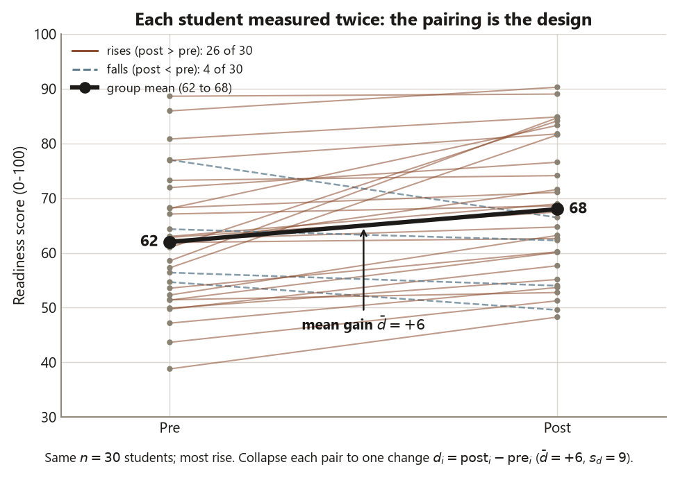
Now both readings are in play, and the temptation is to set the pre-scores beside the post-scores like two groups and compare their means. Resist it. Look at the structure instead. The unit of analysis is the student, and each student carries two numbers that are linked — the post-score that sits next to a given pre-score is the same person’s later reading, not an unrelated observation. That linkage is exactly what an independent two-group analysis assumes away. The design is paired, and the blueprint’s step 2 tells you what to do about it: reduce each student’s pair to a single number, the within-student difference,

\[ d_i = \text{post}_i - \text{pre}_i . \]

Now you have one column of thirty differences, one per student. And a column of thirty numbers with a question about its mean is precisely the one-sample structure from the section above. So the paired \(t\)-test is not a new method at all — it is the one-sample \(t\) procedure run on the differences, testing the mean difference against the reference value \(0\) (“no change”). The whole trick of the paired design is this collapse: two linked readings per unit become one difference per unit, and a two-sample-looking problem becomes a one-sample problem. The method follows from the structure, not from a flowchart of test names.

For Dataset P, the differences have mean \(\bar d = +6.0\) points with standard deviation \(s_d = 9.0\). That \(\bar d = +6\) is the estimate; everything downstream is its uncertainty and its interpretation.

Figure 1: Each student is measured twice — the pairing is the whole design. All \(n = 30\) students carry a pre-score and a post-score joined by a line; most rise (26 of 30 here), and the bold line tracks the group mean climbing from \(62\) to \(68\) — the locked \(\bar d = +6\) gain. This is exactly why you collapse each pair to one within-student change \(d_i = \text{post}_i - \text{pre}_i\) and analyze that single column, rather than comparing two clouds of numbers. Synthetic; seed 35203.

Why pairing reduces variability and raises power

Here is the payoff, and it is worth seeing as a number, not a slogan. The standard error of the mean difference is a one-sample SE on the differences:

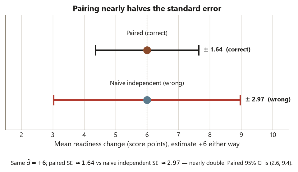
\[ \mathrm{SE}(\bar d) = \frac{s_d}{\sqrt{n}} = \frac{9.0}{\sqrt{30}} \approx 1.64 \text{ points.} \]

Now imagine you had ignored the pairing and treated the pre-scores and post-scores as two independent samples of \(30\). The standard error of the difference in means would then be

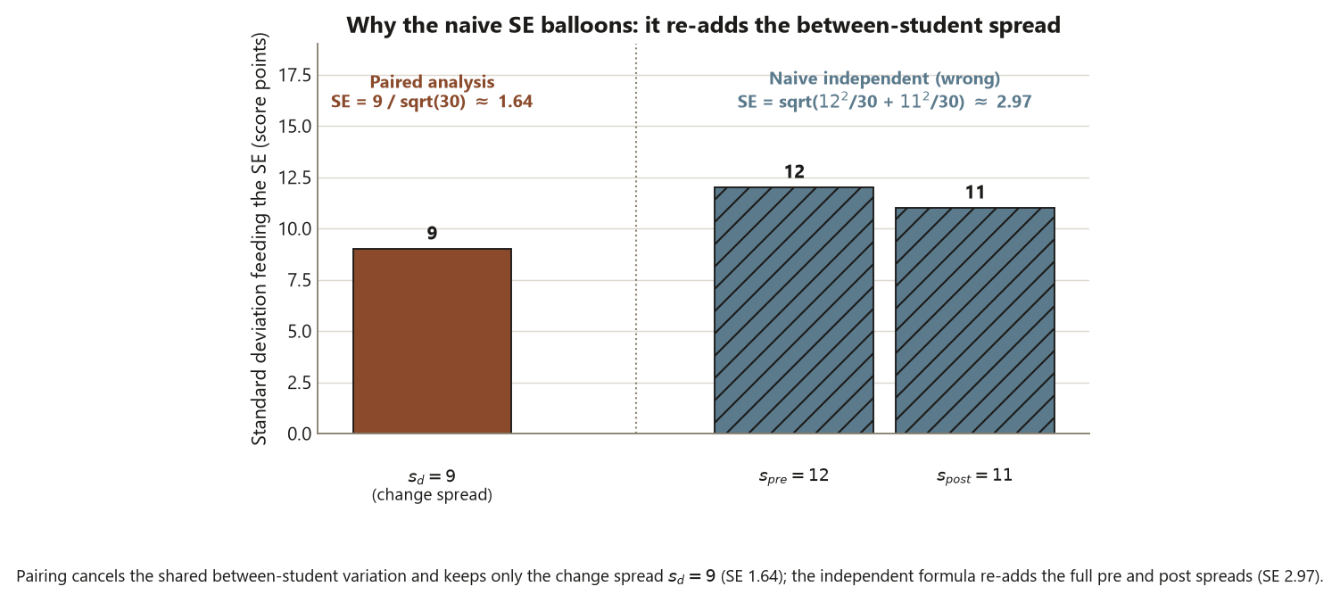
\[ \mathrm{SE}_{\text{indep}} = \sqrt{\frac{s_{\text{pre}}^2}{n} + \frac{s_{\text{post}}^2}{n}} = \sqrt{\frac{12^2}{30} + \frac{11^2}{30}} \approx 2.97 \text{ points.} \]

That is nearly double the paired SE — \(2.97\) against \(1.64\) — for the very same data. Why the gap? Because the independent-samples formula carries the full between-student spread twice (the \(12\) and the \(11\)), while the paired formula carries only the spread of the changes, \(s_d = 9\). Students differ a lot from each other, but each student’s change is far more stable; the differencing cancels the shared between-student variation and leaves only the within-student noise. A smaller SE is a tighter interval and a larger \(t\), so pairing — when the design genuinely is paired — is the more powerful analysis. The naive independent SE is not just a different number; it is the wrong number for this design, and quoting it would understate the precision the pairing actually earned.

Figure 2: Pairing nearly halves the standard error. The same \(+6\)-point estimate is shown twice: with the correct paired standard error (\(\pm 1.64\)) and with the wrongly-independent one (\(\pm 2.97\)). The naive independent bar is nearly twice as wide for the very same data, because it carries the full between-student spread twice while the paired SE carries only the spread of the changes. The locked paired 95% interval is the narrow one, \((2.6, 9.4)\). Synthetic; seed 35203.

With the paired SE in hand, the paired \(t\)-statistic is

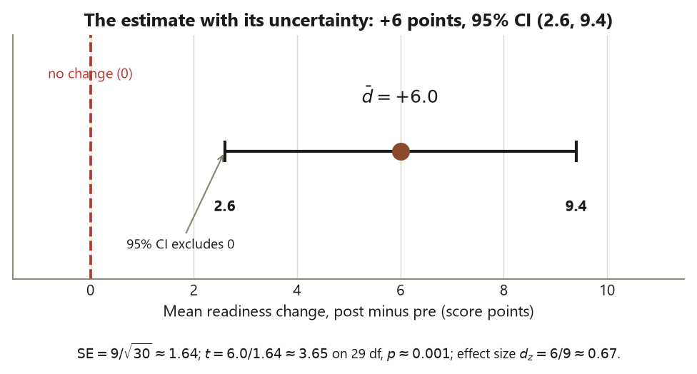
\[ t = \frac{\bar d}{\mathrm{SE}(\bar d)} = \frac{6.0}{1.64} \approx 3.65 \quad \text{on } 29 \text{ df,} \]

with \(p \approx 0.001\). The 95% confidence interval for the true mean change is

\[ \bar d \pm t_{29,\,.975}\,\mathrm{SE}(\bar d) = 6 \pm 2.045(1.64) \approx 6 \pm 3.4 = (2.6,\ 9.4) \text{ points,} \]

and the standardized effect size is

\[ d_z = \frac{\bar d}{s_d} = \frac{6}{9} \approx 0.67 . \]

Read each of these as a blueprint move. The estimate is \(\bar d = +6\) points. Its uncertainty is the interval \((2.6, 9.4)\) — plausible mean gains run from about three points to about nine, and because the interval excludes \(0\), “no change” is implausible (that is the same information the \(p \approx 0.001\) carries, but the interval also tells you the size). The effect size \(d_z \approx 0.67\) says the typical gain is about two-thirds of a difference-standard-deviation — a medium-to-large standardized effect. The conclusion keeps the three things apart: the result is statistically clear, the practical size (\(+6\) on a 100-point scale) is modest-to-meaningful and a judgment call for the program, and — with no control group — this is an improvement over time, not evidence that the module caused it.

Worked examples

Worked example — Dataset P: the paired readiness diagnostic (recurring slice)

Question. Did students’ quantitative-readiness scores change over the six-week support module? Comparing two readings on the same people — a comparison question about a within-student change. Data are synthetic; set.seed(35203).

Structure. The unit is the student (\(n = 30\)). The outcome is quantitative (a 0–100 readiness score). The design is paired — each student is measured before and after, so the two readings are linked. This is not two independent groups. Step 2 of the blueprint says: form the differences.

Method. Reduce each student to one number, \(d_i = \text{post}_i - \text{pre}_i\), and run a one-sample \(t\) procedure on the thirty differences against the reference value \(0\). The differences have \(\bar d = +6.0\) and \(s_d = 9.0\).

Assumptions & diagnostics. The thirty differences are independent (different students); the distribution of the differences should be roughly normal (or \(n = 30\) large enough for the CLT to carry \(\bar d\)). You check this on the differences themselves — a histogram or QQ plot of the \(d_i\) — not on the raw pre/post columns. No extreme outlier in the changes is assumed here.

Estimate & uncertainty. The estimate is \(\bar d = +6.0\) points. The standard error is \(\mathrm{SE} = 9/\sqrt{30} \approx 1.64\), giving \(t = 6.0/1.64 \approx 3.65\) on \(29\) df, \(p \approx 0.001\), and a 95% CI of \((2.6, 9.4)\) points. The standardized effect size is \(d_z = 6/9 \approx 0.67\). The static R below shows both ways to get there — the paired call and the equivalent one-sample call on the differences. It is teaching code and is not executed here.

Figure 3: The paired estimate carried with its uncertainty. The point estimate is \(\bar d = +6.0\) readiness points, and the 95% confidence interval runs from \(2.6\) to \(9.4\) — the whole interval sits above the dashed no-change line at \(0\), so “no gain” is implausible. Reading the interval, not a lone \(p\)-value, is the discipline: plausible mean gains run from about three to about nine points (\(\mathrm{SE} \approx 1.64\), \(t \approx 3.65\) on \(29\) df, \(p \approx 0.001\), \(d_z \approx 0.67\)). Synthetic; seed 35203.

set.seed(35203)

# Dataset P: same 30 students, readiness measured pre and post (synthetic).
# pre  : mean 62, SD ~ 12      post : mean 68, SD ~ 11
# (values summarized to their locked paired summaries for this static slice)

# --- The paired t-test: post vs pre, paired = TRUE -------------------------
t.test(post, pre, paired = TRUE)
#   mean of the differences (post - pre) = 6.0   SE = 1.64
#   t = 3.65   df = 29   p-value ~= 0.001
#   95% CI for the mean difference: (2.6, 9.4) points

# --- The SAME analysis, written as a one-sample t on the differences -------
diff <- post - pre                 # 30 within-student changes; mean d-bar = 6.0
t.test(diff)                       # one-sample t of the differences vs 0
#   mean(diff) = 6.0   SE = s_d/sqrt(n) = 9/sqrt(30) = 1.64
#   t = 3.65   df = 29   p ~= 0.001   95% CI (2.6, 9.4)

d_z <- mean(diff) / sd(diff)       # standardized effect: 6 / 9 ~= 0.67

# --- The locked contrast: what the WRONG (independent) SE would give -------
# Treating pre and post as two independent samples of 30:
#   SE_indep = sqrt(12^2/30 + 11^2/30) ~= 2.97   <- nearly DOUBLE the paired 1.64
# The pairing removes between-student variation, so the paired SE is smaller.

Conclusion. Students gained about six readiness points on average, plausibly between 2.6 and 9.4 (\(d_z \approx 0.67\), a medium-to-large standardized change). Because the interval excludes \(0\) and \(p \approx 0.001\), “no change” is implausible — but report the estimate and its interval, not just the \(p\)-value. The locked SE contrast is the lesson: the honest paired SE is \(1.64\), while the naive independent SE would be \(2.97\), nearly double, understating the precision the pairing earned. And the boundary: with no control group, this is an improvement over six weeks, not proof the module caused it — maturation, test familiarity, and regression to the mean are uncontrolled. Statistical significance, practical size, and causation stay three separate claims.

Worked example — reaction time before and after a short break (transfer, new context)

Question. Does a brief rest change people’s reaction time on a simple task? A within-person comparison. These numbers are illustrative and distinct from Dataset P.

Structure. The unit is the person (\(n = 12\) here). The outcome is quantitative (reaction time in milliseconds). The design is paired — each person is timed before a five-minute break and again after, on the same task. The two readings belong to the same person, which is exactly what licenses the paired analysis. If these had been different people before and after, you would have an independent two-group design and a different SE.

Method. Form each person’s change \(d_i = \text{after}_i - \text{before}_i\) and run a one-sample \(t\) on the twelve differences against \(0\).

Assumptions & diagnostics. The twelve differences are independent (different people); check that the differences look roughly normal with \(n = 12\) — small samples lean harder on that assumption, so a QQ plot of the changes matters more here than it did with \(n = 30\).

Estimate & uncertainty. Suppose the mean change is \(\bar d = -18\) ms (faster after the break) with \(s_d = 24\) ms. Then \(\mathrm{SE} = 24/\sqrt{12} \approx 6.9\) ms, \(t = -18/6.9 \approx -2.6\) on \(11\) df, and a 95% CI of roughly \(-18 \pm 2.20(6.9) \approx (-33, -3)\) ms; the effect size is \(d_z = -18/24 \approx -0.75\).

set.seed(35203)

# Reaction-time trial: same 12 people, before vs after a 5-min break (illustrative).
diff <- after - before              # 12 within-person changes (ms); d-bar = -18
t.test(diff)                        # one-sample t of the differences vs 0
#   mean(diff) = -18 ms   SE = 24/sqrt(12) ~= 6.9
#   t = -2.6   df = 11   95% CI ~ (-33, -3) ms   d_z = -18/24 ~= -0.75

# Equivalent paired call:
t.test(after, before, paired = TRUE)   # same -18 ms mean difference, same CI

Conclusion. People reacted about 18 ms faster after the break, plausibly between roughly \(3\) and \(33\) ms faster (\(d_z \approx -0.75\)). The decisive structural point is the matching: because each person is their own before-and-after, the paired analysis is the correct one, and it cancels the large person-to-person differences in baseline speed. Same blueprint as Dataset P, new context — and the same honesty about limits: with no control condition, “faster after the break” is an association with time, not proof the break caused the speed-up (practice on the task could do the same). Report the estimate and its interval; keep significance, size, and cause distinct.

A common mistake

This week’s classic applied-methods error lives in step 2 of the blueprint — design identification — and it cuts both ways.

The first and most common flavor is analyzing paired data as two independent groups. A student lines up the thirty pre-scores and the thirty post-scores, runs a two-sample (independent) \(t\)-test, and reports the result. The point estimate of the difference comes out the same — \(\bar d = 6\) either way — but the uncertainty is wrong. The independent-samples SE here is about \(2.97\), while the correct paired SE is \(1.64\), nearly half. So the wrong analysis produces a wider interval and a smaller \(t\), throwing away the power the pairing earned and possibly missing a real effect. The fix is not a different formula to memorize; it is to read the structure first. Ask the diagnostic question: is the post-score next to a given pre-score the same unit’s later reading? If yes, the design is paired, you analyze the differences, and you use the one-sample SE on those differences. The design tells you the method.

Figure 4: Why the naive independent SE balloons. The paired standard error is built from a single spread — the spread of the changes, \(s_d = 9\) — giving \(\mathrm{SE} \approx 1.64\). The independent-samples formula instead re-adds the full between-student spreads, \(s_{\text{pre}} = 12\) and \(s_{\text{post}} = 11\) (the hatched bars), the very variation pairing was designed to cancel, giving \(\mathrm{SE} \approx 2.97\). Same data, nearly double the standard error — that is the cost of misreading the design as two independent groups. Synthetic; seed 35203.

The mirror flavor is just as damaging: pairing data that are not actually matched. If the thirty “before” readings and the thirty “after” readings come from different students — a fresh cohort each time — then there are no genuine pairs, the differences you would compute are meaningless arithmetic between unrelated people, and the paired analysis is invalid. You cannot manufacture a pairing by sorting two columns and subtracting; the matching has to be a real feature of how the data were collected (same person, twins, matched cases). The honest discipline is to name the pairing mechanism before you difference anything: what makes observation \(i\) in column one the partner of observation \(i\) in column two? If you cannot answer that with a real link, you do not have paired data, and forcing a paired analysis is as wrong as ignoring a real one. Identify the design honestly — paired because of a stated matching, independent because of separate units — and let that identification, not habit, choose the method.

Low-stakes self-checks (ungraded)

These are for your own practice — ungraded, no submission.

1. In one sentence, state why the paired \(t\)-test on Dataset P is “really” a one-sample procedure, and say what single column of numbers it operates on.
2. The paired SE for Dataset P is \(1.64\) and the naive independent SE is \(2.97\). Explain in one sentence why the paired SE is smaller, using the phrase “between-student variation.”
3. Write the 95% confidence interval for the mean readiness change, and interpret it in a sentence that reports an estimate with uncertainty rather than a bare \(p\)-value.
4. A classmate has thirty “before” scores from one group of students and thirty “after” scores from a different group, and runs a paired \(t\)-test by subtracting column from column. Name what is wrong and what design they actually have.
5. The effect size is \(d_z = 6/9 \approx 0.67\). Say in one sentence what that number means in plain words, and whether it is a statement about statistical or practical significance.
6. The result is statistically clear (\(p \approx 0.001\)). Write one sentence stating what this paired analysis cannot conclude about causation, and name one uncontrolled explanation for the gain.

Reading and source pointer

This week is grounded in the instructor notes (the primary course materials) for the one-sample and paired-comparison framing — forming the differences and running a one-sample procedure on them — with the IMS (Cetinkaya-Rundel & Hardin) treatment of inference for a single mean and paired data for the concept sequence: a point estimate, its standard error, a confidence interval, and the paired-difference setup. Navarro (Learning Statistics with R) is named only as an optional reference for the mechanics of the paired \(t\)-test. These notes are the course’s own synthesis, grounded in but not copied from the sources. No prose, examples, exercises, figures, or solutions are reproduced from any source.

Public vs. graded

These notes, the examples, and the practice here are public and ungraded — study material only. No graded prompts, answer keys, rubrics, point values, or due dates appear on this site. Graded applied-methods checkpoints, weekly quizzes, homework and analysis memos, applied analysis labs, the midterm, the applied methods project, and the final exam live in Blackboard (the LMS), which is authoritative for due dates, submissions, and grades. If this page and Blackboard ever disagree, follow Blackboard.

Looking ahead

Next week the two groups are independent — different students, not the same student twice — so there are no differences to form and no pairing to exploit. You compare the groups directly: the Support cohort against the Self-guided cohort, a difference in means of \(6\) points with its own two-sample standard error (about \(2.38\), via Welch’s \(t\)), its own confidence interval, and its own effect size. The contrast with this week is the whole point: the design changed from paired to independent, and with it the method, the standard error, and what you are licensed to conclude — including a fresh dose of association-versus-causation, because next week’s students chose their condition.

See also

• Week 3 — Estimation, uncertainty & practical significance — the estimate-with-its-interval discipline this week runs on.
• Week 5 — Two-group comparisons — the same six-point gap, but now independent groups and a two-sample SE.
• Method chooser — the question → structure → method decision guide; paired vs. independent is the branch this week turns on.
• Assumptions and diagnostics guide — checking normality of the differences for a paired analysis.
• Methods glossary — paired difference, one-sample \(t\), standard error, \(d_z\).