Lab 8 — ANOVA with multiple comparisons

One-way ANOVA, Tukey HSD, and a planned contrast in R

Purpose. This lab is the hands-on companion to Week 8 — Multiple comparisons and planned contrasts. The note argues that once a one-way ANOVA’s omnibus \(F\) tells you the four instructional formats are not all the same, the honest follow-up question is which formats differ — and that asking all six pairwise questions at once inflates the family-wise error rate unless you control it. Here you build that workflow end to end on Dataset F (final exam score by instructional format): fit the one-way ANOVA with aov(), read the omnibus \(F \approx 7.61\) and the effect size \(\eta^2 \approx 0.19\) off summary(), run TukeyHSD() to see which of the six pairwise gaps clear the honest-significant difference of about \(6.64\) points, and finally test one pre-specified planned contrast — hands-on formats versus delivered-only formats — which estimates \(\hat\psi = 8\) points with \(t \approx 4.44\). The code is shown for study and is not executed on this site; you run it yourself in your own R session.

The idea

A one-way ANOVA answers a deliberately blunt question: across the four instructional formats — Lecture (L), Lecture+Lab (LL), Online (O), and Hybrid (H) — is there any difference in mean final score, or could the four sample means \(L = 74\), \(LL = 81\), \(O = 70\), \(H = 79\) have come from one common population by sampling luck alone? The omnibus \(F\) statistic is the verdict on that single yes/no question. With \(F \approx 7.61\) on \((3, 96)\) degrees of freedom and \(p \approx 0.0001\), the answer is “not all equal” — but notice how little that tells you. It does not say which formats differ, by how much, or whether any gap is large enough to matter to a student deciding how to take the course. The omnibus test opens the door; it does not walk you through it.

Two follow-up moves walk you through it, and they answer two genuinely different questions. The first is exploratory: now that we know the formats are not all alike, which specific pairs differ? There are \(\binom{4}{2} = 6\) pairwise comparisons (L–LL, L–O, L–H, LL–O, LL–H, O–H), and if you tested each one at the usual \(5\%\) level you would be running six tests, so the chance of at least one false alarm across the family climbs well above \(5\%\). Tukey’s Honest Significant Difference (HSD) controls that family-wise error rate: it widens each comparison’s yardstick so that the whole set of six holds at \(5\%\). On Dataset F that yardstick is a critical difference of about \(6.64\) points — a pairwise gap must exceed \(6.64\) to count as honestly significant. Three pairs clear it (LL–O \(= 11\), H–O \(= 9\), LL–L \(= 7\)); three do not (H–L \(= 5\), L–O \(= 4\), LL–H \(= 2\)).

The second follow-up is confirmatory and it is the more powerful move when you have a question in advance. Suppose that before seeing the data you had a specific hypothesis: the two hands-on formats (Lecture+Lab and Hybrid, which add active practice) outperform the two delivered-only formats (plain Lecture and Online, which deliver content without structured practice). That is a single, pre-specified planned contrast — a weighted combination of the four group means whose weights sum to zero, \(\hat\psi = \tfrac{1}{2}(\bar x_{LL} + \bar x_H) - \tfrac{1}{2}(\bar x_L + \bar x_O)\). Because you asked one directed question rather than fishing through all six pairs, the contrast spends none of its power on multiplicity control: it estimates \(\hat\psi = 80 - 72 = 8\) points with \(t \approx 4.44\) and \(p < 0.001\). The discipline to name here is the difference between planned and post-hoc: a contrast you committed to before looking is a sharp, powerful confirmatory test; the same arithmetic run after spotting the pattern in the data is data-dredging and needs the same multiplicity penalty Tukey applies.

Through all three layers — omnibus, Tukey, contrast — keep the course’s two recurring disciplines in view. First, report the estimate with its uncertainty, not a bare verdict: the omnibus \(F\) comes with \(\eta^2 \approx 0.19\) (format explains about \(19\%\) of score variance), each Tukey comparison comes with a confidence interval for the mean gap, and the contrast comes with \(\hat\psi = 8\) points and its standard error, not just a \(p\)-value. Second, keep statistical, practical, and causal significance distinct: an \(8\)-point format gap on a \(100\)-point exam is statistically clear and arguably practically meaningful, but Dataset F is observational in spirit — if students were not randomly assigned to formats, an ANOVA buys you association, not proof that the format caused the score. The arithmetic is the same either way; the causal license depends on the design, not on the size of \(F\).

Goal

By the end of this lab you should be able to:

• Encode the Dataset F final-score-by-format slice in R with a fixed seed, name the student as the unit of analysis, and confirm the four group means are the locked \(L = 74\), \(LL = 81\), \(O = 70\), \(H = 79\).
• Fit the one-way ANOVA with aov(score ~ format) and read the omnibus \(F \approx 7.61\) on \((3, 96)\), \(p \approx 0.0001\), and the effect size \(\eta^2 \approx 0.19\) off the summary() table.
• Run TukeyHSD(), read which of the six pairwise gaps exceed the honest-significant difference of about \(6.64\) points, and report each significant pair as a mean difference with a confidence interval, not just a flag.
• Build and test one pre-specified planned contrast (hands-on LL, H versus delivered-only L, O), obtain \(\hat\psi = 8\) points with \(t \approx 4.44\), and explain why a planned contrast is more powerful than the post-hoc pairwise sweep.
• Reconcile every number against the week-8 note and state, in one sentence, what an ANOVA on observational format data can and cannot conclude.

The point of the lab is the error-rate discipline and the planned-versus-post-hoc distinction, not the R syntax: the omnibus \(F\) poses one question, Tukey controls the family-wise error rate across the six pairwise questions, and a planned contrast answers a single directed question with full power. Name the blueprint move as you go — what is the estimate (a mean gap, an effect size, a contrast value), what is its uncertainty (a confidence interval, a standard error), what is assumed (roughly equal variances, roughly normal residuals, independent students), and what can and cannot be concluded (statistical significance is not practical importance, and observational data buy association, not causation).

Setup

You need base R for the fit (aov, summary, TukeyHSD); the planned contrast is shown two ways — with the emmeans package for the readable idiom, and by hand from the group means so you can see the arithmetic underneath. Every chunk that draws randomness starts with set.seed(35203), the course-wide seed, so your run reproduces the locked Dataset F numbers. The data are synthetic; seed set — these are not real student records.

Fix the design facts before any code runs, because every number below follows from them:

• Unit of analysis: the individual student. There are \(N = 100\) students, \(n = 25\) in each of the four formats; every count below counts students, and the balanced \(25/25/25/25\) design is what makes the contrast standard error so clean.
• Response and factor: the response is the final exam score (\(0\)–\(100\), quantitative); the single grouping factor is instructional format with four levels (L, LL, O, H). One factor, four groups — this is the one-way ANOVA structure.
• What was not randomized: treat Dataset F as observational in spirit — students were not (in this synthetic world) randomly assigned to formats. So a format gap reads as an association with score, not as proof a format caused a higher score; motivated or better-prepared students may self-select into hands-on formats. (Week 11 revisits exactly this by adjusting for a pretest covariate.)
• The locked slice: group means \(L = 74\), \(LL = 81\), \(O = 70\), \(H = 79\); grand mean \(= 76\); common within-group SD \(\approx 9\), so \(\mathrm{MSE} = 81\). Omnibus \(F \approx 7.61\) on \((3, 96)\), \(p \approx 0.0001\), \(\eta^2 \approx 0.19\). Tukey critical difference \(\approx 6.64\). Planned contrast \(\hat\psi = 8\) points, \(t \approx 4.44\), \(p < 0.001\).

set.seed(35203)

# --- Dataset F: final exam score (0-100) by instructional FORMAT ----------------
# Cypress Ridge Student-Success Study. One factor (format), four levels, n = 25
# each, N = 100. Response = final score (quantitative). OBSERVATIONAL in spirit:
# students were not randomly assigned to format, so gaps are ASSOCIATIONS, not
# proven causal effects. Synthetic; seed set; LOCKED group means below.
n_per <- 25                                  # students per format (balanced design)

# Build each format's 25 scores so the GROUP MEAN hits the locked target exactly,
# with a common within-group SD of about 9 (so MSE = 81). rnorm() supplies the
# scatter; we recenter each group to its locked mean so the means are not left to
# sampling luck. (You may instead read a saved data frame with the same means.)
make_group <- function(mu, n = n_per, sd = 9) {
  z <- rnorm(n)                              # raw scatter
  mu + sd * (z - mean(z)) / sd(z)            # recenter/rescale to mean = mu, SD = sd
}

score  <- c(make_group(74),                  # Lecture        (L):  mean 74
            make_group(81),                  # Lecture+Lab   (LL):  mean 81
            make_group(70),                  # Online         (O):  mean 70
            make_group(79))                  # Hybrid         (H):  mean 79
format <- factor(rep(c("L", "LL", "O", "H"), each = n_per),
                 levels = c("L", "LL", "O", "H"))

datF <- data.frame(format, score)

tapply(datF$score, datF$format, mean)        # -> L 74, LL 81, O 70, H 79 (LOCKED)
mean(datF$score)                             # -> 76  (grand mean)
tapply(datF$score, datF$format, sd)          # -> all about 9 (common within-group SD)

The four group means come out at the locked \(L = 74\), \(LL = 81\), \(O = 70\), \(H = 79\), the grand mean at \(76\), and each within-group SD at about \(9\). Those means are the estimates every later step reads from; the recentring step is just bookkeeping so the synthetic scatter does not drift the means off their locked targets. Note the structure already in view: one quantitative response, one four-level factor, balanced cells — the textbook one-way ANOVA layout. Everything below asks two questions about these four means: are they all equal (the omnibus \(F\)), and if not, which differ and by how much (Tukey and the contrast)?

Steps

You will build the multiple-comparisons workflow in four moves: fit the ANOVA and read the omnibus verdict (Step 2), turn that verdict into an effect size (still Step 2), run Tukey HSD to see which pairs honestly differ (Step 3), and test the one planned contrast you committed to in advance (Step 4). Step 1 is the data build above — confirm its means before you go on.

Step 1 — Confirm the locked group means

Before fitting anything, re-run the tapply() check from Setup and make sure the four means are exactly \(74\), \(81\), \(70\), \(79\). The entire lab reads from these four numbers, so a drift here propagates into every later result. This is the cheapest bug to catch.

set.seed(35203)

# Sanity check the data BEFORE the ANOVA: the four group means and the grand mean.
group_means <- tapply(datF$score, datF$format, mean)
group_means                                  # -> L 74, LL 81, O 70, H 79  (LOCKED)
mean(datF$score)                             # -> 76  (grand mean)

# A quick look at the structure you are about to model: side-by-side boxplots.
boxplot(score ~ format, data = datF,
        main = "Final score by instructional format (Dataset F)",
        xlab = "Format", ylab = "Final exam score")

The boxplot is the same “see the structure before you fit it” move from week 2: four groups, visibly different centers (LL and H high, O low, L in the middle), roughly comparable spreads. If your printed means are not the locked four, stop and fix the Setup chunk — the recenter step in make_group() should force each group mean onto its target. The means are what the ANOVA partitions; if they are wrong, the \(F\) statistic will be wrong in a way that looks like a real result, which is exactly the trap to avoid.

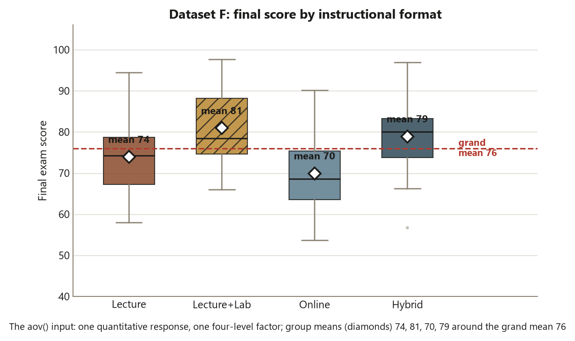
Figure 1: The aov() input — four formats, one response. Side-by-side boxplots of Dataset F final score show the four instructional formats with their locked group means marked as white diamonds: Lecture \(74\), Lecture+Lab \(81\), Online \(70\), Hybrid \(79\), scattered around the dashed grand mean of \(76\). Lecture+Lab (hatched) sits highest and Online lowest; the boxes have visibly different centers but roughly comparable spreads — the balanced, near-equal-variance layout a one-way ANOVA assumes. This is the picture to confirm before fitting anything: if these four centers are not the locked means, the \(F\) that follows is wrong in a way that looks real. Synthetic; seed 35203.

Step 2 — Fit the one-way ANOVA and read the omnibus F and η²

Now fit the model. aov(score ~ format) partitions the total variation in score into a between-format piece (how far the four group means sit from the grand mean) and a within-format piece (scatter of students around their own group mean). The ratio of their mean squares is the \(F\) statistic, and summary() prints the ANOVA table. The effect size \(\eta^2\) — the share of total variation that is between-format — is not in the default table, so compute it from the sums of squares.

set.seed(35203)

# Fit the one-way ANOVA: one quantitative response, one four-level factor.
fitF <- aov(score ~ format, data = datF)
summary(fitF)
#               Df  Sum Sq  Mean Sq  F value   Pr(>F)
# format         3    1850   616.7    7.61    1.0e-04   ***   <- omnibus F (LOCKED)
# Residuals     96    7776    81.0                             <- MSE = 81

# Effect size: eta-squared = SS_between / SS_total (share of variance explained).
ss   <- summary(fitF)[[1]][["Sum Sq"]]       # c(SS_between, SS_within)
eta2 <- ss[1] / sum(ss)                      # 1850 / (1850 + 7776)
round(eta2, 2)                               # -> 0.19  (format explains ~19% of variance)

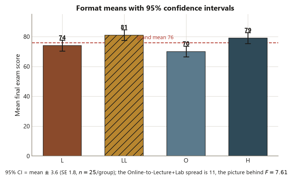
The omnibus verdict is \(F \approx 7.61\) on \((3, 96)\) degrees of freedom with \(p \approx 0.0001\): the four format means are very unlikely to be this spread out if all four populations shared one common mean, so reject the null of equal means. But state the estimate, not just the verdict — that is the first recurring discipline. The effect size \(\eta^2 \approx 0.19\) says instructional format accounts for about \(19\%\) of the variation in final score; the other \(81\%\) is within-format student-to-student variation (the \(\mathrm{MSE} = 81\), a within-group SD of \(9\)). A \(19\%\) share is a moderate, practically meaningful effect — but \(\eta^2\) alone still does not tell you which formats differ, and that is what Steps 3 and 4 are for. And keep the causal discipline in view: a large \(F\) on observational data is strong evidence the formats are associated with different scores, not proof that switching a student’s format would cause the gap.

Figure 2: The estimate behind the omnibus \(F\). The four format means with \(95\%\) confidence intervals: Lecture+Lab (\(81\)) and Hybrid (\(79\)) sit above the dashed grand mean of \(76\), Online (\(70\)) below, and Lecture (\(74\)) between. Each interval is the mean \(\pm 3.6\) (standard error \(1.8\) with \(n = 25\) per group), so the roughly \(11\)-point Online-to-Lecture+Lab spread is comfortably wider than the intervals — the estimate-with-uncertainty picture behind \(F \approx 7.61\) and \(\eta^2 \approx 0.19\). The chart shows that the formats differ and by about how much; it does not yet say which specific pairs are distinguishable, which is what Steps 3 and 4 are for. Synthetic; seed 35203.

Step 3 — Tukey HSD: which pairs honestly differ?

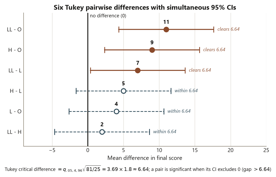
The omnibus test said “not all equal.” Tukey HSD turns that into the six specific pairwise questions while holding the family-wise error rate at \(5\%\). TukeyHSD() reports, for each of the six pairs, the estimated mean difference, a \(95\%\) confidence interval adjusted for all six comparisons, and an adjusted \(p\)-value. A pair is honestly significant when its adjusted interval excludes zero — equivalently, when the gap exceeds the honest-significant difference of about \(6.64\) points.

set.seed(35203)

# Tukey HSD: all six pairwise gaps, with family-wise error held at 5%.
tuk <- TukeyHSD(fitF, conf.level = 0.95)
tuk
#            diff      lwr     upr   p adj
# LL-L       7      ...     ...    <0.05   *   (7 > 6.64  -> significant)
# O-L       -4      ...     ...    n.s.        (4 < 6.64  -> NOT significant)
# H-L        5      ...     ...    n.s.        (5 < 6.64  -> NOT significant)
# O-LL     -11      ...     ...    <0.01   **  (11 > 6.64 -> significant)
# H-LL      -2      ...     ...    n.s.        (2 < 6.64  -> NOT significant)
# H-O        9      ...     ...    <0.01   **  (9 > 6.64  -> significant)

# The honest-significant difference (critical gap) for this balanced design:
q   <- qtukey(0.95, nmeans = 4, df = 96)     # studentized-range critical value ~ 3.69
hsd <- q * sqrt(81 / 25)                     # MSE = 81, n = 25 per group
round(hsd, 2)                                # -> ~ 6.64  (LOCKED critical difference)

Three pairs clear the \(6.64\)-point yardstick and three do not. The significant gaps are LL–O \(= 11\), H–O \(= 9\), and LL–L \(= 7\): Lecture+Lab and Hybrid both beat Online, and Lecture+Lab beats plain Lecture. The non-significant gaps are H–L \(= 5\), L–O \(= 4\), and LL–H \(= 2\) — each falls short of \(6.64\), so once you control the family-wise error you cannot honestly distinguish those pairs from no difference. Report each significant pair as a mean difference with its interval (“Lecture+Lab scored about \(11\) points higher than Online, \(95\%\) CI excluding zero”), never as a bare “significant” stamp — that is the estimate-with-uncertainty discipline applied to multiplicity. The classic error this step prevents: running six unadjusted \(t\)-tests would wrongly flag H–L (\(5\)) or L–O (\(4\)) as significant, because at \(5\%\) each, six tests give roughly a \(1 - 0.95^6 \approx 26\%\) chance of at least one false alarm. Tukey’s wider yardstick is the price of asking six questions at once and still trusting the answer.

Figure 3: Six pairwise gaps against one honest yardstick. Each of the six Tukey pairwise differences is drawn with its simultaneous \(95\%\) confidence interval of \(\pm 6.64\) — the honest-significant difference \(q_{.05,4,96}\sqrt{81/25} = 3.69 \times 1.8 \approx 6.64\). A pair is honestly significant when its interval clears zero: LL–O \(= 11\), H–O \(= 9\), and LL–L \(= 7\) (solid lines, filled points, “clears 6.64”) do; H–L \(= 5\), L–O \(= 4\), and LL–H \(= 2\) (dashed lines, open points, “within 6.64”) do not. Holding the family-wise error at \(5\%\) is exactly what stops the three small gaps from being read as real differences. Synthetic; seed 35203.

Step 4 — A planned contrast: hands-on versus delivered-only

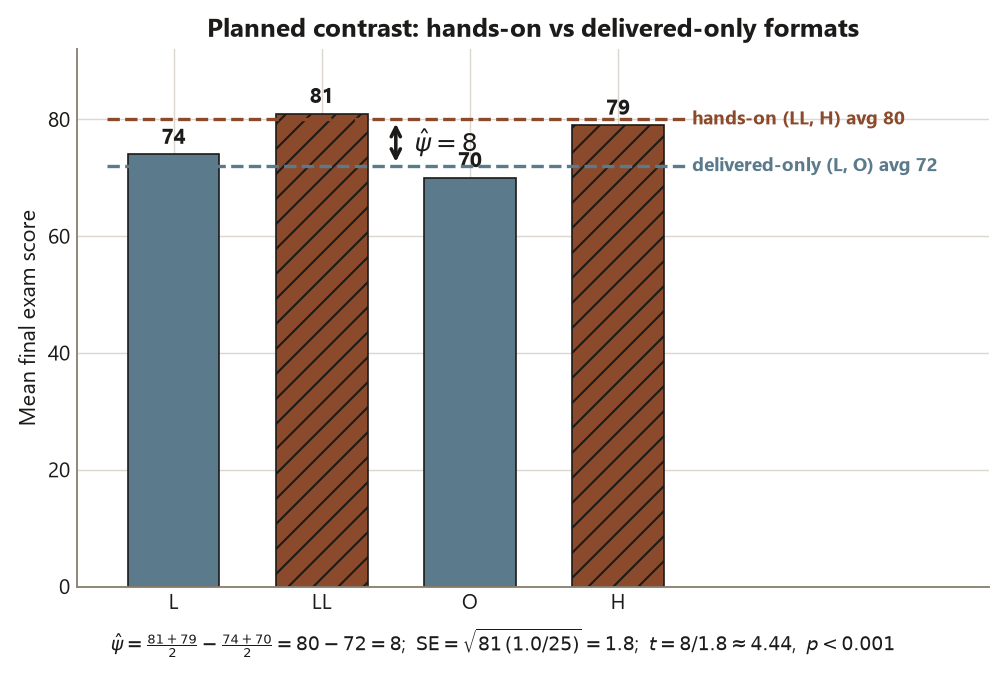
Tukey was exploratory — it scanned all six pairs. Now test the one directed question you committed to before seeing the data: do the two hands-on formats (Lecture+Lab and Hybrid, which add active practice) beat the two delivered-only formats (plain Lecture and Online)? That is a single planned contrast with weights \((c_L, c_{LL}, c_O, c_H) = (-\tfrac12, +\tfrac12, -\tfrac12, +\tfrac12)\) that sum to zero. Because it is one pre-specified question, it carries no multiplicity penalty and is more powerful than the post-hoc sweep. Here it is two ways — the readable emmeans idiom, and the same number by hand.

set.seed(35203)

# --- Planned contrast via emmeans (the readable idiom) -------------------------
library(emmeans)
emm <- emmeans(fitF, ~ format)               # estimated marginal means per format

# Weights line up with the factor levels c("L","LL","O","H"):
#   hands-on  = LL, H  (+1/2 each);  delivered-only = L, O (-1/2 each); sum = 0.
hands_vs_delivered <- contrast(
  emm,
  list("hands-on vs delivered-only" = c(-1/2, +1/2, -1/2, +1/2))
)
hands_vs_delivered
#  contrast                    estimate   SE   df  t.ratio  p.value
#  hands-on vs delivered-only      8     1.8   96   4.44    <0.001   <- LOCKED contrast

# --- The SAME contrast by hand, from the locked group means -------------------
m  <- tapply(datF$score, datF$format, mean)  # L 74, LL 81, O 70, H 79
cw <- c(L = -1/2, LL = 1/2, O = -1/2, H = 1/2)[names(m)]   # align weights to levels
psi_hat <- sum(cw * m)                       # (81 + 79)/2 - (74 + 70)/2 = 80 - 72
psi_hat                                      # -> 8  (LOCKED contrast estimate, points)

se_psi <- sqrt(81 * sum(cw^2) / 25)          # MSE = 81, n = 25; sum(cw^2) = 1.0
t_psi  <- psi_hat / se_psi                   # 8 / 1.8
round(c(SE = se_psi, t = t_psi), 2)          # -> SE 1.80, t 4.44  (LOCKED)

The contrast estimates \(\hat\psi = \tfrac{81 + 79}{2} - \tfrac{74 + 70}{2} = 80 - 72 = 8\) points: the hands-on formats average about \(8\) points higher on the final than the delivered-only formats. Its standard error is \(\mathrm{SE}(\hat\psi) = \sqrt{81 \times 1.0 / 25} = 1.8\), so \(t = 8 / 1.8 \approx 4.44\) on \(96\) df, \(p < 0.001\). Report the estimate with its uncertainty: an \(8\)-point hands-on advantage (roughly \(0.9\) of a within-group SD), clearly distinguishable from zero. Note why this beats the Tukey sweep: by asking one directed question instead of six, the contrast spends no power on multiplicity control, so it can detect the pooled hands-on advantage with a larger, sharper \(t\) than any single pairwise comparison. The discipline to keep straight: this contrast is legitimate only because it was planned. The identical arithmetic run after you spotted that LL and H were the two high groups would be post-hoc data-dredging and would owe the same multiplicity penalty Tukey charges — the weights are honest only if you wrote them down before looking. And once more the causal boundary: an \(8\)-point gap on observational data is an association between format and score, not evidence that assigning a student to a hands-on format would cause an \(8\)-point gain.

Figure 4: One directed question, full power. The planned contrast pools the two hands-on formats (Lecture+Lab \(81\) and Hybrid \(79\), hatched) against the two delivered-only formats (Lecture \(74\) and Online \(70\)): the hands-on average of \(80\) minus the delivered-only average of \(72\) gives \(\hat\psi = 8\). With standard error \(\sqrt{81(1.0/25)} = 1.8\), that is \(t = 8/1.8 \approx 4.44\) on \(96\) df, \(p < 0.001\) — a sharper result than any single Tukey pair, because one pre-specified question spends none of its power on multiplicity control. The double arrow marks the \(8\)-point gap between the two format-group averages; the contrast is legitimate only because it was written down before the data were seen. Synthetic; seed 35203.

Verify

This is the moment where your R run and the week-8 reasoning are supposed to meet. Check each item against the note, and treat any mismatch as a bug in your code, not a discovery about the world — every target value is the locked, synthetic Dataset F slice (illustrative).

• The four group means are \(74\), \(81\), \(70\), \(79\). tapply(datF$score, datF$format, mean) should return \(L = 74\), \(LL = 81\), \(O = 70\), \(H = 79\), and mean(datF$score) should return \(76\). If they drift, the make_group() recenter step in Setup did not fire — re-check it before reading any later number, because every result downstream is computed from these four means.
• The omnibus \(F\) is about \(7.61\) on \((3, 96)\). The summary(fitF) table should show \(\mathrm{Df} = 3\) and \(96\), \(\mathrm{SS}_{\text{between}} = 1850\), \(\mathrm{SS}_{\text{within}} = 7776\), \(\mathrm{MSE} = 81\), and \(F \approx 7.61\) with \(p \approx 0.0001\). A different \(F\) usually means your group means or your \(n\) per group drifted — recheck Step 1.
• The effect size is \(\eta^2 \approx 0.19\). ss[1] / sum(ss) should be about \(1850 / 9626 \approx 0.19\). If you get a wildly different value, confirm you took \(\mathrm{SS}_{\text{between}} / \mathrm{SS} _{\text{total}}\) and not \(\mathrm{SS}_{\text{between}} / \mathrm{SS}_{\text{within}}\).
• The Tukey critical difference is about \(6.64\). qtukey(0.95, 4, 96) * sqrt(81/25) should land near \(3.69 \times 1.8 \approx 6.64\). The three significant pairs must be LL–O \(= 11\), H–O \(= 9\), LL–L \(= 7\); the three non-significant pairs must be H–L \(= 5\), L–O \(= 4\), LL–H \(= 2\). If your significant set differs, you likely read unadjusted \(p\)-values instead of TukeyHSD()’s adjusted ones — the whole point of the step is the family-wise correction.
• The planned contrast is \(\hat\psi = 8\) with \(t \approx 4.44\). Both the emmeans route and the by-hand route should give \(\hat\psi = 8\) points, \(\mathrm{SE} = 1.8\), \(t \approx 4.44\), \(p < 0.001\). If the contrast comes out near zero, your weights are misaligned to the factor levels c("L","LL","O","H") — confirm the hands-on formats (LL, H) carry \(+\tfrac12\) and the delivered-only formats (L, O) carry \(-\tfrac12\), and that the weights sum to zero.
• The conclusion is stated correctly. In one sentence: one-way ANOVA shows the four formats are not all equal (\(F \approx 7.61\), \(\eta^2 \approx 0.19\)); Tukey HSD honestly distinguishes LL and H from O (and LL from L) while holding the family-wise error at \(5\%\); a planned hands-on-versus-delivered-only contrast estimates an \(8\)-point advantage (\(t \approx 4.44\)); and because format was not randomly assigned, all of this is association, not proof of a causal format effect. If your written conclusion reports a bare \(p\)-value without the estimate, calls the format gap causal, or treats the planned contrast as if it were post-hoc, the reasoning — not the code — needs fixing.

A small honest note on what is and is not exact. The omnibus \(F\), \(\eta^2\), the Tukey critical difference, and the contrast \(t\) are all locked, drafted, synthetic targets — they are what the week-8 note reports, not values re-derived live (R is not executed on this site). Because the Setup chunk recenters each group to its locked mean, your group means should match to the digit; the \(F\) and contrast then follow from those means plus the locked \(\mathrm{MSE} = 81\). If a number is off, the fix is almost always upstream in the data build, not in the model call.

AI use note

If you use an AI assistant on this lab, record it briefly. The load-bearing column is Verification — how you confirmed the output yourself, against the week-8 note and the locked numbers, rather than trusting the tool. Computation, AI-assisted or not, does not choose the right multiplicity correction, license a causal claim, or certify a number.

Tool	Purpose	Verification
LLM chat assistant	Explain why TukeyHSD() widens the yardstick relative to six unadjusted \(t\)-tests	Re-ran Step 3, confirmed the critical difference qtukey(0.95,4,96)*sqrt(81/25) \(\approx 6.64\), and checked that only LL–O, H–O, LL–L clear it; reconciled against the week-8 note’s significant-pairs list
LLM chat assistant	Confirm the planned-contrast weights are aligned to the factor levels c("L","LL","O","H")	Verified the by-hand psi_hat (\(= 8\)) matched the emmeans estimate, that the weights summed to zero, and that LL, H carried \(+\tfrac12\) and L, O carried \(-\tfrac12\); reconciled with Setup
LLM chat assistant	Clarify the difference between a planned contrast and a post-hoc comparison	Restated in my own words that the \(t \approx 4.44\) is honest only because the contrast was pre-specified, and that the same arithmetic post-hoc would owe a multiplicity penalty; checked against the note
Code formatter / linter	Tidy the make_group() and contrast blocks for readability	Diffed before/after to confirm only whitespace changed; re-checked that the printed group means stayed \(74, 81, 70, 79\) and the contrast stayed \(\hat\psi = 8\)

See also

• Week 8 — Multiple comparisons and planned contrasts — the companion note: why the omnibus \(F\) is only the opening question, how Tukey controls the family-wise error rate, and why a planned contrast beats the post-hoc sweep.
• Week 6 — Many-group comparisons and one-way ANOVA — where the omnibus \(F \approx 7.61\) and \(\eta^2 \approx 0.19\) on Dataset F first appear.
• Week 7 — Assumptions, diagnostics, and the midterm — the equal-variance and normal-residual checks that license the ANOVA you fit here.
• Method chooser — the question → structure → method guide: when many group means call for ANOVA plus multiple comparisons.
• Methods glossary — one-way ANOVA, omnibus \(F\), \(\eta^2\), Tukey HSD, family-wise error rate, planned contrast, planned vs post-hoc.
• Reporting and interpretation guide — reporting an effect size with a confidence interval, and keeping statistical, practical, and causal significance distinct.

The graded deliverable, its rubric, and due date live in Blackboard (the LMS) — this page is study and practice only.