Week 1 — Vector spaces over a field, subspaces, and direct sums

Where this week starts

In the prerequisite course a vector was a column of real numbers, and nearly every question became a question about a matrix: row reduce it, count the pivots, decide whether the system was consistent. The fluency that course built is exactly what you will use to check the abstractions below. But it told you what those particular vectors do. It never told you what a vector is.

This week supplies the definition, and the definition points the other way. A vector space is a set with two operations obeying eight axioms, over a field \(F\) fixed in advance. Nothing in that sentence mentions columns, entries, or numbers, so polynomials, matrices, functions, and a set with eight elements over a two-element field are all vector spaces — and a theorem proved from the axioms holds in every one of them at once.

Three things should feel different by the end of the week. The field is a parameter, not a constant: every statement below carries an implicit “over \(F\)”, and twice this page shows a claim true over \(\mathbb{Q}\) or \(\mathbb{R}\) and false over \(\mathbb{F}_2\). A subspace is interesting for how it sits inside its parent, not in isolation. And “sum” and “direct sum” are two different claims about a pair of subspaces; confusing them is the most productive error available this week.

One bookkeeping note. Dimension is not yet a theorem — that every basis of a space has the same size is Week 2’s central work — so where this page writes “dimension three” it means only “here is an evident spanning list of three vectors with no redundancy”, and no argument below leans on a count. Week 2 measures what this week builds, Week 3 maps between the objects, and Week 4 puts a basis on a map to recover the matrix you started with.

Why this matters beyond the definition

Here is the mistake this week exists to prevent. Someone notices that in \(\mathbb{R}^3\) the \(xy\)-plane and the \(yz\)-plane together produce every vector, writes \(\mathbb{R}^3 = U + X\), and concludes that each vector has an “\(xy\)-part” and a “\(yz\)-part”. They then define an operation sending a vector to its \(xy\)-part. That operation does not exist: \((1,2,3)\) equals \((1,2,0) + (0,0,3)\) and it also equals \((1,0,0) + (0,2,3)\), with the first term in the \(xy\)-plane and the second in the \(yz\)-plane both times.

The failure matters because splitting a space so that each vector has exactly one expression is how projections are built, how an operator is broken into simpler operators, and how the eigenvalue theory later in this course decomposes a space into invariant pieces. Every one of those needs the uniqueness, not merely the covering. The direct sum condition is the hypothesis that supplies it, and this week you learn to check it.

What you will be able to do

• State the vector space axioms over an arbitrary field \(F\), and decide whether a given set with given operations satisfies them.
• Prove \(0 \cdot v = 0\) and \((-1) \cdot v = -v\) from the axioms, naming the axiom behind each step.
• Apply the subspace criterion, and exhibit a subset that fails it for a stated reason.
• Prove that \(\operatorname{span}(S)\) is the smallest subspace containing \(S\), and that an intersection of subspaces is a subspace while a union generally is not.
• Prove the three descriptions of an internal direct sum equivalent, and use whichever is cheapest in a given case.
• Exhibit two distinct complements of one subspace, and explain why a complement is never canonical.

Terms and notation worth fixing

Symbol	What it means in this course
\(F\)	the field of scalars, fixed before anything else is said; concretely \(\mathbb{R}\), \(\mathbb{Q}\), \(\mathbb{C}\), or \(\mathbb{F}_2\)
\(V\)	the vector space under study, always over the fixed \(F\)
\(U\), \(X\), \(Y\)	subspaces of \(V\); \(S\) and \(T\) are reserved for linear maps from Week 3 on, so \(S\) appears only as a plain subset inside \(\operatorname{span}(S)\)
\(\{0\}\)	the zero subspace, whose one element is the zero vector; not the empty set
\(\operatorname{span}(S)\)	all finite linear combinations of vectors drawn from \(S\), with \(\operatorname{span}(\emptyset) = \{0\}\)
\(U + X\)	the sum \(\{\, u + x : u \in U,\ x \in X \,\}\), a subspace of \(V\)
\(U \oplus X\)	the same set, written this way only once the sum is known to be direct
\(U \times X\)	the external direct sum: ordered pairs \((u,x)\) with componentwise operations

The axioms and the work the field does

Each axiom below is a rule you may cite by name inside a proof, and this week you will cite them by name until the habit sticks. Read the list once for shape, then read the subsection after it, where the axioms prove facts that look too obvious to need proving.

The eight axioms, and why \(F\) must be a field

Fix a field \(F\). A vector space over \(F\) is a set \(V\) with an addition \(V \times V \to V\) and a scalar multiplication \(F \times V \to V\) satisfying the eight axioms below. Axioms A1, A2, and A5 through A8 are required for all \(u, v, w \in V\) and all \(a, b \in F\); A3 posits one zero vector that works for every \(v\) at once, and A4 then supplies an inverse for each individual \(v\).

\[ \begin{aligned} &\text{(A1)} && u + v = v + u &&\text{(A2)} && (u + v) + w = u + (v + w) \\ &\text{(A3)} && \text{there is } 0 \in V \text{ with } v + 0 = v \text{ for all } v \in V \\ &\text{(A4)} && \text{each } v \in V \text{ has } -v \in V \text{ with } v + (-v) = 0 \\ &\text{(A5)} && a(u + v) = au + av &&\text{(A6)} && (a + b)v = av + bv \\ &\text{(A7)} && (ab)v = a(bv) &&\text{(A8)} && 1 \cdot v = v \end{aligned} \]

Axioms A1 through A4 say \(V\) is an abelian group under addition; A5 through A8 say the field acts on that group compatibly with its own addition, its own multiplication, and its own identity. Nothing here says the elements of \(V\) are numbers, and nothing yet says \(V\) has a basis.

Why must \(F\) be a field and not merely a commutative ring? Because of cancellation. Suppose \(av = 0\) with \(a \ne 0\) in \(F\). Then \[ v = 1 \cdot v = (a^{-1}a)v = a^{-1}(av) = a^{-1} \cdot 0 = 0, \] using A8, the existence of \(a^{-1}\) in \(F\), A7, and a fact proved just below. Over a ring this collapses. The ring \(\mathbb{Z}\) acting on the two-element group \(\mathbb{Z}/2\mathbb{Z}\) satisfies all eight axioms verbatim, yet \(2 \cdot 1 = 0\) with \(2 \ne 0\) and \(1 \ne 0\), and that object has no basis of any size. Division by nonzero scalars is used constantly from here on — in this week’s halving trick, in Week 2’s row operations, in every rescaling of a basis vector — so we insist on a field, and say so wherever it matters.

What the axioms force, proved rather than assumed

The facts below are usually waved through. Deriving them is how you learn that the axioms are a working tool.

The zero vector is unique. If \(0\) and \(0'\) both satisfy A3, then \(0 = 0 + 0' = 0' + 0 = 0'\), by A3 for \(0'\), then A1, then A3 for \(0\). So writing “the” zero vector is justified.

Additive inverses are unique. If \(v + w = 0\) and \(v + w' = 0\), then \[ w = w + 0 = w + (v + w') = (w + v) + w' = 0 + w' = w', \] by A3, the second hypothesis, A2, A1 with the first hypothesis, and A3 again. So \(-v\) names one specific vector.

Scalar zero kills every vector: \(0 \cdot v = 0\). The left \(0\) is the zero of \(F\) and the right one is the zero vector; the notation deliberately does not distinguish them. By A6 with \(a = b = 0\) in the field, \[ 0 \cdot v = (0 + 0) \cdot v = 0 \cdot v + 0 \cdot v . \] Add \(-(0 \cdot v)\), which exists by A4, to both sides and regroup with A2 and A3: the left side becomes \(0\) and the right side becomes \(0 \cdot v\). The same argument run through A5 gives \(a \cdot 0 = 0\) for every scalar \(a\).

Multiplying by \(-1\) inverts: \((-1) \cdot v = -v\). Compute \[ v + (-1)v = 1 \cdot v + (-1)v = (1 + (-1))v = 0 \cdot v = 0, \] by A8, then A6, then the previous fact. So \((-1)v\) is an additive inverse of \(v\), and by uniqueness it is \(-v\). Note what is not happening: \(-v\) is not defined as \((-1)v\). The inverse comes from A4 and the scalar \(-1\) comes from the field, and the content is that they agree.

Four spaces to carry through the block

\(F^n\): column vectors of length \(n\) over \(F\), added and scaled entrywise. This is the space the prerequisite course studied, with \(F = \mathbb{R}\).

\(P_3(F)\): polynomials in one variable over \(F\) of degree at most three, added and scaled coefficientwise. The subscript is the degree bound, so \(1, x, x^2, x^3\) is an evident spanning list and \(\dim P_3(F) = 4\), not three. Treat these as formal polynomials, determined by their four coefficients, rather than as functions. Over \(\mathbb{F}_2\) that distinction has teeth: \(x\) and \(x^2\) are different elements of \(P_3(\mathbb{F}_2)\) but define the same function, since \(0^2 = 0\) and \(1^2 = 1\).

\(M_2(F)\): two-by-two matrices over \(F\) with entrywise operations, so \(\dim M_2(F) = 4\), spanned by the four matrices with a single \(1\). Matrix multiplication plays no part in the vector space structure.

\(\mathbb{F}_2^3\): triples over the two-element field \(\mathbb{F}_2 = \{0,1\}\), where \(1 + 1 = 0\). There are exactly \(2^3 = 8\) vectors, and every one satisfies \[ v + v = 1 \cdot v + 1 \cdot v = (1 + 1)v = 0 \cdot v = 0, \] so each vector is its own additive inverse and subtraction is addition. If you were trained over \(\mathbb{R}\) that will feel wrong for a while; it is simply what the axioms say in characteristic two. Week 2 adds the sequences \(F^{\mathbb{N}}\) as the block’s infinite-dimensional example.

Subspaces, spans, and two ways to combine them

A subspace of \(V\) is a subset that is itself a vector space under the operations \(V\) already carries. Checking eight axioms for each candidate would be intolerable and is also unnecessary, since most of them are inherited from the parent for free. What actually has to be checked is short, and the rest of this section builds the tools for combining subspaces once you have them.

The subspace criterion, and a set that fails it

Criterion. Let \(V\) be a vector space over \(F\) and let \(U \subseteq V\) be nonempty, closed under addition, and closed under scalar multiplication. Then \(U\) is a subspace of \(V\).

Argument. Commutativity, associativity, both distributive laws, \((ab)v = a(bv)\), and \(1 \cdot v = v\) are statements about elements; they hold for all vectors of \(V\), hence for those lying in \(U\). That leaves A3 and A4. Since \(U\) is nonempty, choose \(u \in U\); scalar closure gives \(0 \cdot u \in U\), and \(0 \cdot u = 0\) was proved above, so the zero vector lies in \(U\). For A4, given \(v \in U\), closure gives \((-1)v \in U\), and \((-1)v = -v\). Both missing axioms follow from the two closures plus nonemptiness.

Nonemptiness cannot be dropped: the empty set is vacuously closed under both operations and has no zero vector. The two closures also compress into one — a nonempty \(U\) with \(au + bv \in U\) for all \(a, b \in F\) and \(u, v \in U\) is a subspace — which is usually the fastest form to check.

Now a set that fails. Inside \(\mathbb{R}^2\) take \(U = \mathbb{Z}^2\), the vectors with integer entries. It contains \(0\) and is closed under addition, but \(\tfrac{1}{2}(1,0) = (\tfrac{1}{2},0)\) has left the set, so scalar closure fails. A failure of a different kind: \(Y = \{(x,y) \in \mathbb{R}^2 : y = x + 1\}\) is a straight line, but \(0 \notin Y\), so A3 fails at once. Since every subspace contains the zero vector, that is the cheapest test to run first.

The field decides which conditions carry content. Over \(\mathbb{F}_2\) the only scalars are \(0\) and \(1\); scalar closure asks that \(0 \cdot u = 0\) lie in \(U\) and that \(1 \cdot u = u\) lie in \(U\), and the second is automatic. So a subset of an \(\mathbb{F}_2\)-space is a subspace exactly when it contains \(0\) and is closed under addition. Over \(\mathbb{R}\) that shortcut is false, as \(\mathbb{Z}^2\) shows.

Span as the smallest subspace containing a set

Let \(S \subseteq V\) be any subset. Define \(\operatorname{span}(S)\) to be the set of all finite linear combinations \(a_1 s_1 + \cdots + a_k s_k\) with \(k \ge 0\), each \(a_i \in F\) and each \(s_i \in S\); the empty combination is the zero vector, so \(\operatorname{span}(\emptyset) = \{0\}\). Finiteness is not a technicality. The axioms supply an addition of two vectors and nothing else, so an infinite sum has no meaning here. This definition is used unchanged for the rest of the course, including in infinite-dimensional spaces.

Proposition. \(\operatorname{span}(S)\) is a subspace containing \(S\), and it is contained in every subspace of \(V\) that contains \(S\). So it is the smallest such subspace, and equals the intersection of all of them.

Argument. It contains \(0\), so it is nonempty. A sum of two finite combinations from \(S\) is another one, obtained by concatenating the lists, and \(a(a_1 s_1 + \cdots + a_k s_k) = (aa_1)s_1 + \cdots + (aa_k)s_k\) by A5 and A7, so the criterion applies. Each \(s \in S\) equals \(1 \cdot s\) by A8, so \(S \subseteq \operatorname{span}(S)\). Now let \(U\) be any subspace with \(S \subseteq U\): scalar closure puts each \(a_i s_i\) in \(U\), and additive closure applied \(k-1\) times puts the whole combination in \(U\), so \(\operatorname{span}(S) \subseteq U\). Being the least element of the collection of subspaces containing \(S\) is the same as being their intersection.

Intersections behave; unions do not

Proposition. If \(U\) and \(X\) are subspaces of \(V\), so is \(U \cap X\); the same holds for any family of subspaces.

Argument. The zero vector lies in every subspace, so the intersection is nonempty. If \(v, w\) lie in both, then \(v + w\) lies in both and \(av\) lies in both, since each subspace is closed under the two operations. Nothing in the argument used finiteness of the family.

Unions are a different story. In \(\mathbb{R}^2\) let \(U = \operatorname{span}\{(1,0)\}\) and \(X = \operatorname{span}\{(0,1)\}\). Both \((1,0)\) and \((0,1)\) lie in \(U \cup X\), but \((1,0) + (0,1) = (1,1)\) lies on neither line. The general statement is sharp.

Proposition. \(U \cup X\) is a subspace if and only if \(U \subseteq X\) or \(X \subseteq U\).

Argument. If one contains the other, the union is the larger one. Conversely, suppose \(U \cup X\) is a subspace and \(U \not\subseteq X\). Pick \(u \in U\) with \(u \notin X\), and let \(x \in X\) be arbitrary. Then \(u + x \in U \cup X\). If \(u + x\) were in \(X\), then \(u = (u + x) - x\) would lie in \(X\), contradicting the choice of \(u\); so \(u + x \in U\), and therefore \(x = (u + x) - u \in U\). As \(x\) was arbitrary, \(X \subseteq U\).

This is why containment is only a partial order on subspaces: two of them need not be comparable, and when they are not, the union is the wrong way to combine them.

Five subspaces of R three arranged by containment, two of them incomparable.

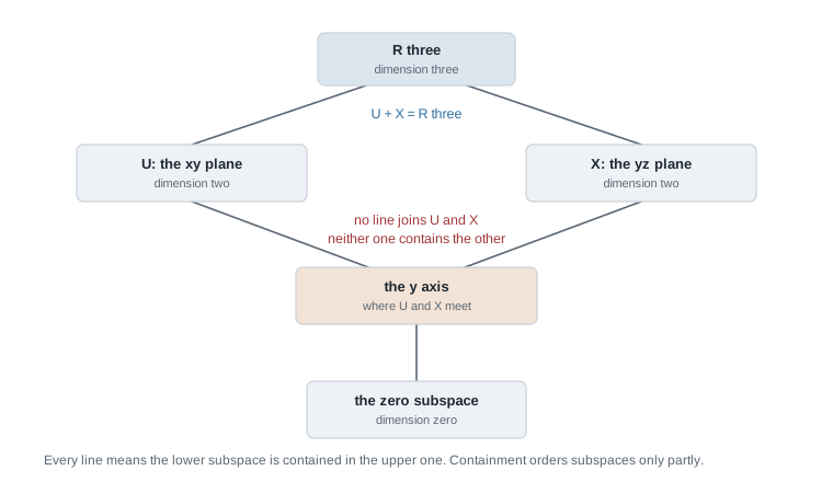
Reading the diagram upward, each line means the lower subspace is contained in the upper one. The two planes sit at the same level with no line between them, because neither contains the other. Below them, the largest subspace inside both is the \(y\)-axis; above them, the smallest subspace containing both is all of \(\mathbb{R}^3\). That upper one is what the next subsection names.

When a sum is direct: three statements that agree

Since unions fail, define instead \[ U + X = \{\, u + x : u \in U, \ x \in X \,\}. \] This is a subspace: it contains \(0 = 0 + 0\), the sum \((u + x) + (u' + x') = (u + u') + (x + x')\) regroups by A1 and A2, and \(a(u+x) = au + ax\) by A5. In fact \(U + X = \operatorname{span}(U \cup X)\), so it is the smallest subspace containing both — the join at the top of the diagram above.

Now the week’s central result. Three conditions of quite different flavour — one about uniqueness, one about an intersection, one about a single vector — turn out to be one condition.

Theorem. Let \(U\) and \(X\) be subspaces of a vector space \(V\) over \(F\). The following are equivalent.

1. Every \(v \in U + X\) has exactly one expression \(v = u + x\) with \(u \in U\) and \(x \in X\).
2. \(U \cap X = \{0\}\).
3. The only way to write \(0 = u + x\) with \(u \in U\) and \(x \in X\) is \(u = 0\) and \(x = 0\).

When these hold the sum is direct, written \(U \oplus X\); if in addition \(U + X = V\) we write \(V = U \oplus X\) and call \(X\) a complement of \(U\) in \(V\). No finite-dimensionality is assumed in the statement or in the proof.

Argument. We prove \((1) \Rightarrow (3) \Rightarrow (2) \Rightarrow (1)\).

Assume (1). The vector \(0\) lies in \(U + X\) and has the expression \(0 + 0\) with \(0 \in U\) and \(0 \in X\). If also \(0 = u + x\) with \(u \in U\) and \(x \in X\), uniqueness forces \(u = 0\) and \(x = 0\).

Assume (3), and let \(v \in U \cap X\). Then \(v \in U\) and \(-v = (-1)v \in X\), the latter by closure of \(X\) under scalar multiplication. So \(0 = v + (-v)\) has the required shape, and (3) forces \(v = 0\). Since \(0\) lies in both subspaces anyway, \(U \cap X = \{0\}\).

Assume (2), and suppose \(u + x = u' + x'\) with \(u, u' \in U\) and \(x, x' \in X\). Rearranging gives \(u - u' = x' - x\). The left side lies in \(U\) and the right side in \(X\), and they are the same vector, so it lies in \(U \cap X = \{0\}\); hence \(u = u'\) and \(x = x'\). Existence of at least one expression is the definition of \(U + X\).

Which condition you use is a matter of convenience: (2) is usually cheapest by hand, (3) generalises cleanly to sums of three or more subspaces, and (1) is the property you actually wanted. Note what the theorem does not say: nothing about whether \(U + X\) is all of \(V\). Directness and covering are independent, and this week’s two worked examples pull them apart in both directions.

Complements exist, and there are many of them

Every subspace of \(\mathbb{R}^3\) has a complement, and the cases are all visible: the complement of \(\{0\}\) is \(\mathbb{R}^3\) and conversely, a line \(\operatorname{span}\{u\}\) with \(u \ne 0\) has as complement any plane through the origin missing \(u\), and a plane has as complement any line through the origin not lying in it. The general theorem — every subspace of a finite-dimensional space has a complement — is proved in Week 2 by extending a basis of \(U\) to a basis of \(V\). That is the one step this page compresses, because the tool it needs does not exist yet.

Non-uniqueness is already visible in dimension two, and it is the more important point. In \(\mathbb{R}^2\) let \(U = \operatorname{span}\{(1,0)\}\) and consider \[ X_1 = \operatorname{span}\{(0,1)\}, \qquad X_2 = \operatorname{span}\{(1,1)\}. \] Both are complements. For \(X_1\): any \((a,b)\) equals \(a(1,0) + b(0,1)\), so \(U + X_1 = \mathbb{R}^2\); and if \(c(1,0) = d(0,1)\) then comparing entries gives \(c = d = 0\), so \(U \cap X_1 = \{0\}\). For \(X_2\): any \((a,b)\) equals \((a-b)(1,0) + b(1,1)\), so \(U + X_2 = \mathbb{R}^2\); and if \(d(1,1) \in U\) its second entry \(d\) is \(0\), so \(U \cap X_2 = \{0\}\). Yet \(X_1 \ne X_2\), since \((1,1) \notin X_1\).

One line in R two with two different complements, splitting the same vector two ways.

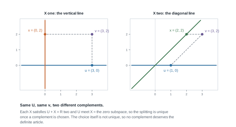
The figure tracks \(v = (3,2)\) through both choices. With \(X_1\) the splitting is \((3,2) = (3,0) + (0,2)\); with \(X_2\) it is \((3,2) = (1,0) + (2,2)\), since \((3,2) = 1 \cdot (1,0) + 2 \cdot (1,1)\). Each splitting is unique once the complement is fixed — the theorem guarantees exactly that — but the choice of complement is not forced by \(U\). So a complement is never “the” complement, and you should distrust any construction that quietly assumes it is. In particular nothing this week licenses the phrase “orthogonal complement”: orthogonality needs an inner product, and this course has not put one on \(V\).

The external direct sum

The sum \(U + X\) presupposes that both already sit inside a common space. When they do not, build a new one. Given vector spaces \(U\) and \(X\) over the same field \(F\), the external direct sum \(U \times X\) is the set of ordered pairs with \[ (u, x) + (u', x') = (u + u', x + x'), \qquad a(u,x) = (au, ax). \] All eight axioms are checked componentwise, the zero vector is \((0,0)\), and the inverse of \((u,x)\) is \((-u,-x)\). Nothing requires \(U\) and \(X\) to be related, so \(\mathbb{R}^2 \times P_3(\mathbb{R})\) is a perfectly good space. If they do sit inside one \(V\), the rule \((u,x) \mapsto u + x\) sends \(U \times X\) onto \(U + X\), and by condition 1 it is one-to-one exactly when the internal sum is direct. An internal direct sum is thus the case where the external construction has already happened inside \(V\).

Worked example — symmetric plus skew matrices over a field

Let \(V = M_2(F)\) and let \[ U = \{ A \in M_2(F) : A^{\mathsf{T}} = A \}, \qquad X = \{ A \in M_2(F) : A^{\mathsf{T}} = -A \}, \] the symmetric and the skew-symmetric matrices, where \(A^{\mathsf{T}}\) is the transpose. Is \(M_2(F) = U \oplus X\)? The honest answer depends on the field.

Step 1: both are subspaces. Transposition satisfies \((A + B)^{\mathsf{T}} = A^{\mathsf{T}} + B^{\mathsf{T}}\) and \((aA)^{\mathsf{T}} = aA^{\mathsf{T}}\). So if \(A, B \in U\) then \((A+B)^{\mathsf{T}} = A^{\mathsf{T}} + B^{\mathsf{T}} = A + B\) and \((aA)^{\mathsf{T}} = aA^{\mathsf{T}} = aA\), and the zero matrix is symmetric, so \(U\) is nonempty. The same computation gives \(X\): if \(A^{\mathsf{T}} = -A\) and \(B^{\mathsf{T}} = -B\) then \((A+B)^{\mathsf{T}} = -A - B = -(A+B)\) and \((aA)^{\mathsf{T}} = a(-A) = -(aA)\).

Step 2: assume \(2 \ne 0\) in \(F\), and split. The hypothesis is that \(2 = 1 + 1\) is invertible in \(F\), which holds in \(\mathbb{Q}\), \(\mathbb{R}\), and \(\mathbb{C}\) and fails in \(\mathbb{F}_2\). Write \(\tfrac12\) for \(2^{-1}\). For any \(A\), \[ A = \tfrac12\left(A + A^{\mathsf{T}}\right) + \tfrac12\left(A - A^{\mathsf{T}}\right). \] The first term is symmetric, since \((A + A^{\mathsf{T}})^{\mathsf{T}} = A^{\mathsf{T}} + A\); the second is skew, since \((A - A^{\mathsf{T}})^{\mathsf{T}} = A^{\mathsf{T}} - A = -(A - A^{\mathsf{T}})\). So \(M_2(F) = U + X\).

Step 3: the sum is direct. If \(A \in U \cap X\) then \(A = A^{\mathsf{T}} = -A\), so \(2A = 0\), and multiplying by \(2^{-1}\) gives \(A = 0\). Condition 2 holds, so \(M_2(F) = U \oplus X\) and every matrix has exactly one symmetric-plus-skew expression.

Step 4: check the count and one instance. A symmetric matrix has entries \(a\), \(b\), \(b\), \(c\) reading across the rows, so three free scalars. A skew one has zero diagonal, because \(a = -a\) gives \(2a = 0\) and hence \(a = 0\), and its off-diagonal entries are \(b\) and \(-b\), so one free scalar: \(3 + 1 = 4 = \dim M_2(F)\). Over \(\mathbb{Q}\), take \[ A = \begin{pmatrix} 1 & 2 \\ 3 & 4 \end{pmatrix}, \qquad A^{\mathsf{T}} = \begin{pmatrix} 1 & 3 \\ 2 & 4 \end{pmatrix} . \] Then \(A + A^{\mathsf{T}} = \begin{pmatrix} 2 & 5 \\ 5 & 8 \end{pmatrix}\) and \(A - A^{\mathsf{T}} = \begin{pmatrix} 0 & -1 \\ 1 & 0 \end{pmatrix}\), so \[ A = \begin{pmatrix} 1 & \tfrac52 \\ \tfrac52 & 4 \end{pmatrix} + \begin{pmatrix} 0 & -\tfrac12 \\ \tfrac12 & 0 \end{pmatrix}, \] and adding entrywise returns \(1\), then \(\tfrac52 - \tfrac12 = 2\), then \(\tfrac52 + \tfrac12 = 3\), then \(4\). The halves are unavoidable, which is the field hypothesis showing up in the arithmetic.

A dimension bar of length four splitting as three plus one, and the same bar collapsing over the two element field.

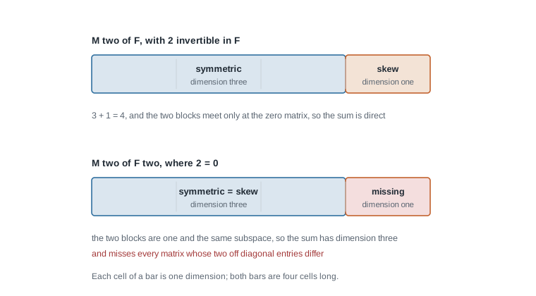
Step 5: where it fails over \(\mathbb{F}_2\). In \(\mathbb{F}_2\) we have \(-1 = 1\), so the condition \(A^{\mathsf{T}} = -A\) says exactly \(A^{\mathsf{T}} = A\). Symmetric and skew are the same condition and \(U = X\). Then \(U \cap X = U \ne \{0\}\), so condition 2 fails outright, and \(U + X = U\) is only the eight symmetric matrices among the sixteen matrices of \(M_2(\mathbb{F}_2)\). Concretely, reduce the entries above modulo two to get \(\begin{pmatrix} 1 & 0 \\ 1 & 0 \end{pmatrix}\), whose transpose is \(\begin{pmatrix} 1 & 1 \\ 0 & 0 \end{pmatrix}\). It is not symmetric, so it lies outside \(U + X\) and has no symmetric-plus-skew expression at all. The lower bar in the figure is that situation: the two blocks have collapsed onto each other and one dimension is unreachable.

The usual repair does not rescue this case either. In characteristic two the structurally correct notion is an alternating matrix, with \(A^{\mathsf{T}} = -A\) and zero diagonal; in \(M_2(\mathbb{F}_2)\) those have entries \(0\), \(b\), \(b\), \(0\), and every one of them is symmetric. The sum is still \(U\) and still misses half the space. The obstruction is arithmetic in the field, not a bad choice of definition.

The same reasoning, transferred

Run the identical argument on functions. Let \(V\) be all functions \(f \colon \mathbb{R} \to \mathbb{R}\) with pointwise operations, a vector space over \(\mathbb{R}\); let \(U\) be the even functions, \(f(-t) = f(t)\), and \(X\) the odd ones, \(f(-t) = -f(t)\). Both are subspaces by the same one-line closure check. For any \(f\), set \[ g(t) = \tfrac12\bigl(f(t) + f(-t)\bigr), \qquad h(t) = \tfrac12\bigl(f(t) - f(-t)\bigr). \] Then \(g\) is even, \(h\) is odd, and \(g + h = f\). If \(f\) is both, then \(f(t) = -f(t)\) for every \(t\), so \(2f(t) = 0\) and \(f = 0\): the sum is direct and \(V = U \oplus X\). For \(f(t) = t^3 + t^2 + 1\) this gives \(g(t) = \tfrac12\bigl((t^3 + t^2 + 1) + (-t^3 + t^2 + 1)\bigr) = t^2 + 1\) and \(h(t) = \tfrac12(2t^3) = t^3\), which do add back to \(f\).

The skeleton stayed the same. In both cases there is an operation \(\sigma\) on \(V\) with \(\sigma(u+v) = \sigma(u) + \sigma(v)\), \(\sigma(av) = a\sigma(v)\), and \(\sigma(\sigma(v)) = v\) — transposition in one case, precomposition with \(t \mapsto -t\) in the other — and the halving trick splits \(V\) into the vectors fixed by \(\sigma\) and those negated by it. Week 3 will call such a \(\sigma\) a linear map. What changed is only the space: \(M_2(F)\) has an evident spanning list of four elements while the function space has no finite one at all, and the theorem never needed one. What would break is the same: halving needs \(2^{-1}\), and in characteristic two the conditions \(\sigma(v) = v\) and \(\sigma(v) = -v\) coincide.

Second worked example — two planes whose sum is not direct

Now pull the other condition away. In \(V = \mathbb{R}^3\) let \(U\) be the \(xy\)-plane and \(X\) the \(yz\)-plane: \[ U = \{(a, b, 0) : a, b \in \mathbb{R}\}, \qquad X = \{(0, b, c) : b, c \in \mathbb{R}\}, \] both subspaces by the closure criterion applied entrywise.

The sum is everything. For any \((a,b,c)\), write \((a,b,c) = (a,b,0) + (0,0,c)\); the first term is in \(U\) and the second in \(X\), its first entry being zero. So \(U + X = \mathbb{R}^3\) and the covering condition holds in full.

The sum is not direct. A vector lies in \(U \cap X\) exactly when its third entry vanishes, because it is in \(U\), and its first entry vanishes, because it is in \(X\). So \(U \cap X = \{(0,b,0) : b \in \mathbb{R}\}\), the \(y\)-axis. That is not \(\{0\}\), so condition 2 fails and therefore condition 1 fails too: some vector has more than one expression.

Two decompositions of one vector. For \(v = (1,2,3)\), \[ (1,2,3) = (1,2,0) + (0,0,3) = (1,0,0) + (0,2,3), \] with the first term of each pair in \(U\) and the second in \(X\), and \((1,2,0) \ne (1,0,0)\). There is in fact a whole line of decompositions, one for each \(t \in \mathbb{R}\): \[ (1,2,3) = (1,t,0) + (0,2-t,3), \] and the freedom is exactly the \(y\)-axis, which is \(U \cap X\). That is the general pattern: once the intersection is nonzero, the decompositions of any fixed vector form a set as large as the intersection.

Two planes in R three crossing along the y axis, with one vector split two ways.

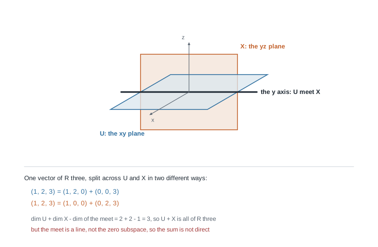
The figure shows both planes, the line where they cross, and the two splittings of \((1,2,3)\). It also records the arithmetic Week 2 will justify: \(\dim U + \dim X - \dim(U \cap X) = 2 + 2 - 1 = 3\), which is \(\dim \mathbb{R}^3\). Two two-dimensional subspaces of a three-dimensional space cannot avoid each other, since \(2 + 2 = 4\) exceeds \(3\); the overlap is forced by arithmetic before any picture is drawn. Compare the same \(U\) with the \(z\)-axis \(Y = \{(0,0,c)\}\): there \(U + Y = \mathbb{R}^3\) and \(U \cap Y = \{0\}\), so \(\mathbb{R}^3 = U \oplus Y\). The only difference between the two situations is the size of the intersection.

The misreading to avoid

The misreading, in the words students actually use, is “\(U + X = V\), so \(V\) is the direct sum of \(U\) and \(X\)”. It is false, and the second worked example is the counterexample: in \(\mathbb{R}^3\) the two planes do sum to everything, and the sum is not direct, because \((1,2,3)\) has infinitely many decompositions. The symbol \(\oplus\) is not a synonym for \(+\); it is \(+\) together with a claim that must be verified separately. Whenever you write \(\oplus\), you owe the reader one of the three equivalent conditions.

The reverse misreading is just as common: “\(U \cap X = \{0\}\), so \(U + X = V\)”. Also false. In \(\mathbb{R}^3\) let \(U\) be the \(x\)-axis and \(X\) the \(y\)-axis. They meet only at the origin, so the sum is direct — but \(U \oplus X\) is the \(xy\)-plane, and no vector with a nonzero third entry belongs to it. Directness controls uniqueness and says nothing about reach. Together these two examples show both failures: covering without uniqueness, and uniqueness without covering. Week 2 supplies the arithmetic that decides when both hold, through \(\dim(U + X) = \dim U + \dim X - \dim(U \cap X)\) for finite-dimensional subspaces.

A third misreading is quieter and does more damage later. Having found one complement of \(U\), students start saying “the complement” and treat “the part of \(v\) lying in \(X\)” as though \(U\) determined it. The two-complements figure refutes that: the same \(U\) and the same \(v\) give \((3,0)\) under one choice and \((1,0)\) under another. A decomposition is determined by the pair \((U, X)\), never by \(U\) alone.

Practice on your own

These are for your own checking, not for submission. Work them with the axioms in front of you.

1. Prove that a nonempty \(U \subseteq V\) with \(au + bv \in U\) for all \(a,b \in F\) and \(u,v \in U\) is a subspace. Then decide whether “nonempty” may be replaced by “\(0 \in U\)”, and whether it may be dropped.
2. In \(\mathbb{F}_2^3\), list every subspace; there are sixteen, namely \(\{0\}\), seven of dimension one, seven of dimension two, and the whole space. Pick two of dimension two, compute their intersection and their sum, and say whether that sum is direct.
3. In \(P_3(F)\) let \(U = \{p : p(0) = 0\}\) and let \(X\) be the constants. Prove \(P_3(F) = U \oplus X\) over any field, using each of conditions 1, 2, and 3 in turn, and say which was shortest.
4. Exhibit two distinct complements of the plane \(\{(a,b,0)\}\) in \(\mathbb{R}^3\) and prove each works. Then do the same for \(\operatorname{span}\{(1,1,0)\}\), which is harder because the obvious coordinate choices are gone.
5. Find subspaces \(U\), \(X\), \(Y\) of \(\mathbb{R}^2\) with \(U + (X \cap Y) \ne (U + X) \cap (U + Y)\); three distinct lines through the origin suffice. What does the failure of that distributive law say about the lattice drawn above?

Where to read more

• MIT OpenCourseWare 18.700 Linear Algebra is the closest open match to this course’s proof-based approach; its opening sessions cover this page’s ground over \(\mathbb{R}\) rather than over a general field.
• MIT OpenCourseWare 18.06 Linear Algebra is the computational complement. Use it when a concrete column-vector picture would help you trust an abstract statement.
• Linear Algebra Done Wrong (Treil) develops abstract vector spaces from the axioms and is a good second exposition of this week.
• The optional Roman alignment for this week is Chapter 1, in the sections on vector spaces, subspaces, and direct sums. That text is optional throughout the course, a borrowed or library copy is sufficient, and nothing here is reproduced from it. Availability and licence terms for every reference above are as stated by their hosts and have not been independently confirmed.
• The course pages: the syllabus, the schedule, the resources page, and the notes overview.

Where this goes next

Every argument on this page avoided counting, which was deliberate and is also a limitation. We could prove a sum direct, but could not decide whether two given subspaces of \(\mathbb{R}^5\) must intersect, and had to defer the claim that every subspace has a complement. Both are counting problems, and counting needs a notion of size independent of how the space was presented.

Week 2 supplies it: linear independence and bases first, then the exchange lemma, which makes dimension well defined rather than merely plausible, then the dimension formula for \(\dim(U + X)\) and with it a purely arithmetic test for directness that settles this week’s misreading. Keep \(P_3(F)\), \(M_2(F)\), and \(\mathbb{F}_2^3\) in mind, since all three return immediately. The notes overview has the shape of the whole four-week block.