Week 6 — Beyond proportions, and posterior predictive thinking
Where this week starts
For three weeks the course has run on one model: forty seeds in a tray, twenty-six of them up, and a Beta prior meeting a binomial likelihood to give a Beta posterior. That model earned its attention, but it left you with a fair suspicion, that the tidy arithmetic of Week 4 was a lucky accident of proportions.
It is not an accident, and this week does the same thing twice more on quantities that are not proportions at all: a campus help desk that wants an arrival rate, a count per unit of time, and a commuter who wants an average trip length. Neither quantity is a probability and neither likelihood is binomial, yet both updates come out in closed form, and both posterior means are the weighted compromise you already know how to read.
Then the week turns to what is genuinely new. Every posterior so far has described a parameter you will never observe directly: the germination rate, the call rate, the mean trip time. What you observe is data, such as how many calls arrive in the next hour. Turning a posterior about a parameter into a distribution over the next observation is a separate move with a separate name, the posterior predictive distribution, and it is always wider than the posterior it came from. By the end of this page you should see two intervals for this week’s help desk, 3.71 to 6.48 and 1 to 10, and say without hesitating which is which and why the second has to be wider.
Why this matters outside the classroom
The help desk has to decide how many staff to put on the phones. Suppose someone reads the posterior for the call rate, sees a 95 percent credible interval of 3.71 to 6.48 calls per hour, and treats its upper end as the busy case to plan for. That looks careful. It is not: the interval says where the long-run average rate probably sits, and a single hour scatters around whatever the rate is. Next hour’s count reaches 10 calls inside its central 95 percent, and even a plan built for eight calls is overrun with probability 0.0775.
The same confusion runs the other way in reporting. A commuter who says the mean trip is between 24.21 and 31.48 minutes has said something true about the commute in general and something worthless about whether to leave at 7:40 tomorrow, for which the honest range is 11.75 to 43.94 minutes. Presenting the first when someone asked the second is how a correct analysis produces a bad decision.
What you will be able to do
- Update a Gamma prior on a rate with Poisson count data, and a normal prior on a mean with normal data of known spread, showing the shape, rate, and precision arithmetic.
- Compute each posterior mean as a weighted average of a prior guess and a data summary, and check that the two weights reproduce the number.
- Distinguish in plain language a posterior for a parameter from a posterior predictive distribution for a new observation, and say which question each answers.
- Derive a predictive distribution’s extra width from its two sources: uncertainty about the parameter, and variation of a single outcome around it.
- Run and interpret an informal posterior predictive check, stating when it is informative and what a passing check does not license.
Terms and notation worth fixing
| Symbol or term | What it means in this course |
|---|---|
| \(\lambda\) | a rate parameter for counts, here calls per hour at the help desk |
| \(s, r\) | the shape and rate of a Gamma distribution, written Gamma\((s, r)\), with mean \(s/r\) |
| \(\mu\) | a mean parameter, here the commuter’s average trip time in minutes |
| \(\sigma\) | the observation-level standard deviation, the spread of single outcomes around \(\mu\) |
| \(\tilde y\) | a new, not-yet-observed outcome the fitted model is asked to predict |
| \(p(\tilde y \mid y)\) | the posterior predictive distribution of \(\tilde y\) given the data already seen |
| precision | one divided by a variance; precisions add, which makes the normal update easy |
| \(T(y)\) | a test quantity: one number computed from a data set and compared across replicates |
One habit of reading saves time all week: whenever you meet a distribution, ask what varies in it, a parameter or a data value.
Two more conjugate models, one shared shape
Learning a second and third conjugate model is worthwhile not because you will meet these exact situations often, but because seeing the same algebra land three times turns a trick into a pattern, and a pattern is what you carry into Week 7 when the closed forms run out. Both models below are set up the same way: name the unknown, state a prior, write the likelihood with the data held fixed, then multiply and read off what is left.
Counts over time: the gamma-Poisson model
The Northgate help desk logs calls. The natural model for a count over an interval is the Poisson distribution: if calls arrive at rate \(\lambda\) per hour and that rate does not change over the shift, the number arriving in \(t\) hours is Poisson with mean \(\lambda t\). The unknown \(\lambda\) is positive, so its prior must live on the positive half-line, where the Gamma family is standard.
The course’s prior here is Gamma(shape 3, rate 2), with mean \(3/2 = 1.5\) calls per hour and standard deviation \(\sqrt{3}/2 = 0.866\); its rate value of 2 makes it worth about two hours of watching. Say what that asserts before looking at data: roughly one or two calls an hour. It is weak, and as you will see it is badly aimed.
Then the shift. Over an \(8\)-hour shift, \(47\) calls arrive, so the observed rate is \(47/8 = 5.875\) calls per hour, nearly four times the prior guess. The likelihood, as a function of \(\lambda\) with the count held fixed, is \(p(y \mid \lambda) \propto \lambda^{47} e^{-8\lambda}\): how plausible is each candidate rate, given 47 calls in eight hours. The Gamma\((s, r)\) prior density is proportional to \(\lambda^{s-1} e^{-r\lambda}\), so multiplying and collecting exponents gives
\[p(\lambda \mid y) \;\propto\; \lambda^{3-1} e^{-2\lambda} \cdot \lambda^{47} e^{-8\lambda} \;=\; \lambda^{(3+47)-1} e^{-(2+8)\lambda}.\]
That is a Gamma density with shape \(3 + 47 = 50\) and rate \(2 + 8 = 10\). The rule is as plain as the beta-binomial one: add the total count to the shape, add the total exposure time to the rate. The posterior mean is \(50/10 = 5.0\) exactly, the mode is \(49/10 = 4.9\), and the standard deviation is \(\sqrt{50}/10 = 0.7071\).
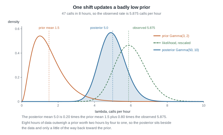
The posterior is nowhere near the prior, because eight hours of counting outweigh a prior worth two hours by four to one, and the weighted check confirms it: \(0.20 \times 1.5 + 0.80 \times 5.875 = 0.3 + 4.7 = 5.0\), the weights being prior rate and observed time as fractions of their total.
Everything worth reporting follows from Gamma(50, 10): a central 95 percent credible interval of 3.711 to 6.478 calls per hour, a posterior median of 4.967, and direct probability statements such as \(P(\lambda > 5.5 \mid y) = 0.2322\) and \(P(\lambda > 6 \mid y) = 0.0844\). That last one is a statement about the rate itself.
# Gamma-Poisson update: Gamma(shape 3, rate 2) prior, 47 calls over an 8-hour shift.
shape_post <- 3 + 47      # 50
rate_post  <- 2 + 8       # 10
shape_post / rate_post                             # posterior mean
qgamma(c(0.025, 0.975), shape_post, rate_post)     # 95 percent credible interval
1 - pgamma(6, shape_post, rate_post)               # posterior probability the rate exceeds 6
A mean with known spread: the normal-normal model
Now a quantity on a continuous scale. A commuter wants \(\mu\), the mean morning trip time in minutes. Trip-to-trip variation is treated as known at \(\sigma = 8\) minutes, a real assumption: mornings scatter around the average with a standard deviation of eight minutes, and that scatter does not itself need estimating. Sixteen trips are timed and average \(\bar y = 27.5\) minutes. The prior is normal with mean 30 and standard deviation 5: the commuter thinks the average is around half an hour and would be mildly surprised below 20 or above 40.
The update is easiest in terms of precision, one over the variance, which measures how much information a distribution carries. Precisions add, and the posterior mean is the precision-weighted average of the prior mean and the sample mean:
\[\text{prior precision} = \frac{1}{5^2} = 0.04, \qquad \text{data precision} = \frac{n}{\sigma^2} = \frac{16}{64} = 0.25.\]
Adding gives a posterior precision of 0.29, so the posterior variance is \(1/0.29 = 3.4483\) and the posterior standard deviation is 1.8570 minutes. The posterior mean is
\[\frac{0.04 \times 30 + 0.25 \times 27.5}{0.29} = \frac{1.2 + 6.875}{0.29} = \frac{8.075}{0.29} = 27.845 \text{ minutes}.\]
Data precision grows with \(n\) and shrinks with \(\sigma^2\). Sixteen trips carry precision 0.25, six and a quarter times the prior’s 0.04, so the posterior mean sits much closer to 27.5 than to 30. The posterior is exactly normal, so its 95 percent credible interval is \(27.845 \pm 1.96 \times 1.857\), from 24.21 to 31.48 minutes.
The pattern all three updates share
Put the three models on one line and the family resemblance is unmissable: each posterior mean is a weighted average of a prior guess and a data summary, with weights that are prior strength and data size as fractions of their total.
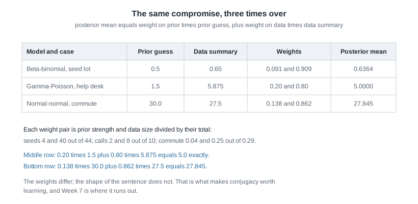
Week 4’s seed lot combined 0.5 with 0.65, weighting them \(4/44 = 0.0909\) and \(40/44 = 0.9091\) to give 0.6364. The help desk combines 1.5 and 5.875 with weights 0.20 and 0.80 to give exactly 5.0. The commute combines 30.0 and 27.5 with weights \(0.04/0.29 = 0.138\) and \(0.25/0.29 = 0.862\): \(0.138 \times 30 + 0.862 \times 27.5 = 4.14 + 23.705 = 27.845\). Three families, one sentence.
The pattern also tells you when each method is informative: when the prior family genuinely describes what you believe and the likelihood genuinely describes how the data arose. The gamma-Poisson update assumes calls arrive independently at an unchanging rate; the normal-normal update assumes independent trips around a fixed mean with a known spread. Both are checkable, and one of them fails later on this page.
Predicting a new observation, not just a parameter
Everything so far produced a distribution over something you cannot see: nobody has ever observed a call rate. What the desk observes is a number of calls in an hour, and the manager’s real question is how many calls to be ready for, not what \(\lambda\) is. If you knew \(\lambda\) exactly, a new hour’s count would be Poisson with mean \(\lambda\). You do not know it; you have a posterior. So average the Poisson distribution over every value \(\lambda\) could take, weighting each by its posterior plausibility:
\[p(\tilde y \mid y) \;=\; \int p(\tilde y \mid \lambda)\, p(\lambda \mid y)\, d\lambda .\]
The words matter more than the integral: the posterior predictive distribution is the model’s distribution for a new observation, averaged over everything you still do not know about the parameter. It is not the likelihood at a best estimate, nor the posterior rescaled. Here the integral has a closed form: averaging a Poisson over a Gamma\((s, r)\) posterior gives a negative binomial with size \(s\) and probability \(r/(r+1)\), so size 50 and probability \(10/11\), with mean 5.0 and standard deviation 2.345 calls.
Where the extra width comes from
The two standard deviations, 0.7071 for the rate and 2.345 for next hour’s count, sit on the same scale and differ by a factor of about 3.3. Do not take that on faith: the variance splits into two pieces you can compute.
\[\operatorname{Var}(\tilde y \mid y) = \underbrace{E[\lambda \mid y]}_{\text{Poisson noise}} + \underbrace{\operatorname{Var}(\lambda \mid y)}_{\text{uncertainty about the rate}} = 5.0 + 0.5 = 5.5 .\]
The first term is 5.0 because a Poisson variance equals its mean; the second is \(\operatorname{Var}(\lambda \mid y) = 50/10^2 = 0.5\), the square of 0.7071. Their sum is 5.5, and \(\sqrt{5.5} = 2.345\). The extra width is not a safety margin: it is Poisson variation that would be there even if you knew \(\lambda\) perfectly, plus the admission that you do not.
It also tells you which term you can shrink. More data drives \(\operatorname{Var}(\lambda \mid y)\) toward zero, so the predictive standard deviation falls toward \(\sqrt{5.0} = 2.236\) and stops there. Predictive intervals narrow to a floor, because the remaining spread is the world, not your ignorance.
Reading the two intervals side by side
Now put both distributions on one axis and read them.
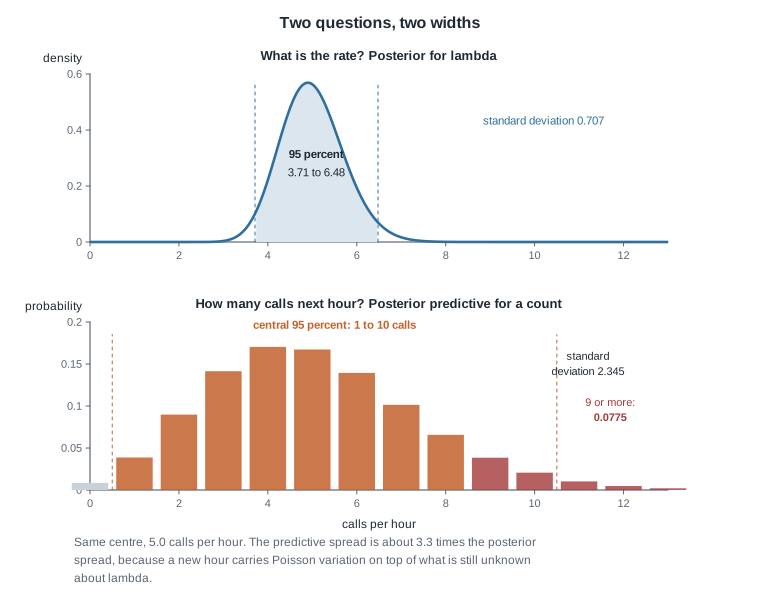
The top panel is the posterior for \(\lambda\), with a central 95 percent interval of 3.711 to 6.478. The sentence it licenses: given this model and this prior, there is a 95 percent posterior probability that the desk’s average arrival rate lies between about 3.7 and 6.5 calls per hour.
The bottom panel is the predictive distribution for one new hour, with a central 95 percent interval of 1 to 10 calls, and its sentence is different: there is at least a 95 percent posterior predictive probability that next hour’s count falls between 1 and 10. That interval is a set of whole numbers, asymmetric because a count cannot be negative.
Two numbers make it concrete: \(P(9 \text{ or more calls in the next hour} \mid y) = 0.0775\), roughly one hour in thirteen, and the probability of a completely quiet hour is \((10/11)^{50} = 0.0085\), what a negative binomial with size 50 and probability \(10/11\) puts on a count of zero. Both are statements about hours, not rates, and neither can be read off the credible interval.
Worked example — the help desk’s next hour
Here is the whole week’s move on one case, from prior to a decision-relevant probability, with every number shown. The Northgate help desk wants its call rate and a staffing plan for the coming hour.
Step 1. Name the unknown and state the prior. The unknown is \(\lambda\), the arrival rate in calls per hour, assumed constant across the shift. The prior Gamma(shape 3, rate 2) has mean 1.5.
Step 2. Write the likelihood. Over eight hours the count is Poisson with mean \(8\lambda\), so 47 calls give a likelihood proportional to \(\lambda^{47} e^{-8\lambda}\).
Step 3. Update. Add the count to the shape and the exposure to the rate: shape 50, rate 10, posterior Gamma(50, 10).
Step 4. Summarize the posterior. Mean \(50/10 = 5.0\); mode 4.9; standard deviation 0.7071; median 4.967; central 95 percent credible interval 3.711 to 6.478. The weighted check \(0.20 \times 1.5 + 0.80 \times 5.875 = 5.0\) holds.
Step 5. Move to the prediction. Averaging Poisson over Gamma(50, 10) gives a negative binomial with size 50 and probability \(10/11\), mean 5.0 and variance \(5.0 + 0.5 = 5.5\), so standard deviation 2.345, and a central 95 percent predictive interval of 1 to 10 calls.
Step 6. Report what was asked. The manager wants the risk of being swamped, here nine or more calls in an hour. That probability is 0.0775.
# Posterior predictive for one new hour, from Gamma(50, 10).
size_pp <- 50
prob_pp <- 10 / 11
qnbinom(c(0.025, 0.975), size = size_pp, prob = prob_pp)   # predictive interval, in calls
1 - pnbinom(8, size = size_pp, prob = prob_pp)             # probability of 9 or more calls
dnbinom(0, size = size_pp, prob = prob_pp)                 # probability of a quiet hour
What this licenses, and what it does not. It licenses saying that under this model a plan built for eight calls an hour is overrun about eight percent of the time. It does not license saying the rate “is” 5.0: that is a posterior mean, and 3.711 to 6.478 is part of the result. Nor does it make 0.0775 a verdict. Whether one hour in thirteen is acceptable weighs a caller waiting against a staffed seat, and no posterior contains that judgment.
The same reasoning, transferred
Run the identical structure on the commute. The unknown \(\mu\) is a mean in minutes rather than a rate, and the posterior from the precision arithmetic above is normal with mean 27.845 and standard deviation 1.8570, giving a 95 percent credible interval of 24.21 to 31.48 minutes.
Now predict one new trip. The predictive distribution is again normal, centred at the same 27.845, with the two variances added as before: observation variance \(\sigma^2 = 64\) plus posterior variance 3.4483 gives 67.4483, so the predictive standard deviation is \(\sqrt{67.4483} = 8.213\) minutes and the 95 percent predictive interval is \(27.845 \pm 1.96 \times 8.213\), from 11.75 to 43.94 minutes.
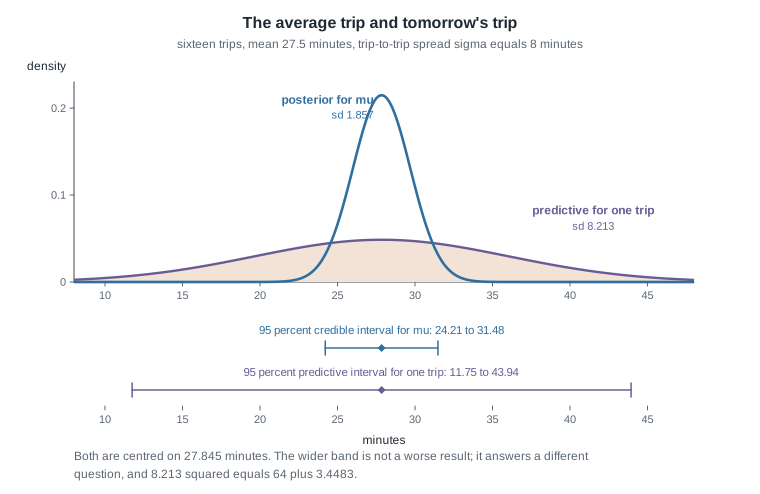
What stayed the same: name the unknown, state a prior, write a likelihood, update in closed form, summarize, then average the sampling distribution over the posterior to predict. What changed: the families, the units, and the algebraic form of the extra width. For counts it was \(E[\lambda \mid y] + \operatorname{Var}(\lambda \mid y)\); here it is \(\sigma^2 + \operatorname{Var}(\mu \mid y)\). Both are observation noise plus parameter uncertainty, and in both the second term is smaller: 3.4483 against 64 here, 0.5 against 5.0 for the calls. Sixteen trips pinned the average down and left the variability of mornings untouched.
# Normal-normal update and prediction for the commute.
sigma <- 8; n <- 16; ybar <- 27.5
prec_prior <- 1 / 5^2
prec_data  <- n / sigma^2
post_mean  <- (prec_prior * 30 + prec_data * ybar) / (prec_prior + prec_data)
post_sd    <- sqrt(1 / (prec_prior + prec_data))
pred_sd    <- sqrt(post_sd^2 + sigma^2)
qnorm(c(0.025, 0.975), post_mean, post_sd)   # credible interval for the mean trip
qnorm(c(0.025, 0.975), post_mean, pred_sd)   # predictive interval for one trip
Second worked example — a busy hour the model did not expect
Everything above assumed the desk’s calls arrive at one constant rate all shift long, an assumption never checked. Checking it is the week’s first taste of what Week 11 makes rigorous.
The idea. A fitted model claims it could have produced data like yours, so take it at its word. Generate replicated data sets from it, the same size and shape as the real one, compute a feature of each, and see where the real data’s value of that feature falls among them. Such a feature is a test quantity, written \(T(y)\).
The real data, hour by hour. The 47 calls did not arrive evenly. The shift log reads 3, 4, 5, 6, 5, 7, 4, 13, which sums to 47 and averages 5.875. Seven hours look like a desk running around five calls an hour. The eighth had 13.
The test quantity. Take \(T(y)\) to be the busiest single hour, so \(T(y) = 13\). The shift total would be a poor choice here, because the update already used it, so comparing it back is circular. The busiest hour is a feature the update never targeted, and exactly the feature a constant-rate assumption would distort.
The replication. Draw a rate from the posterior Gamma(50, 10), draw eight Poisson counts at that rate, record the largest, and repeat.
set.seed(20260906)
lambda_draws <- rgamma(10000, shape = 50, rate = 10)
busiest <- sapply(lambda_draws, function(lam) max(rpois(8, lam)))
mean(busiest >= 13)     # how often a replicated shift is as lopsided as the real one
hist(busiest)
What comes out. A run of 10,000 replicated shifts put about 2.6 percent of them at a busiest hour of 13 or more; most peak between seven and ten calls. The same negative binomial gives 0.0034 for a particular pre-specified hour reaching 13; the busiest-of-eight figure is larger because you get eight chances at it.
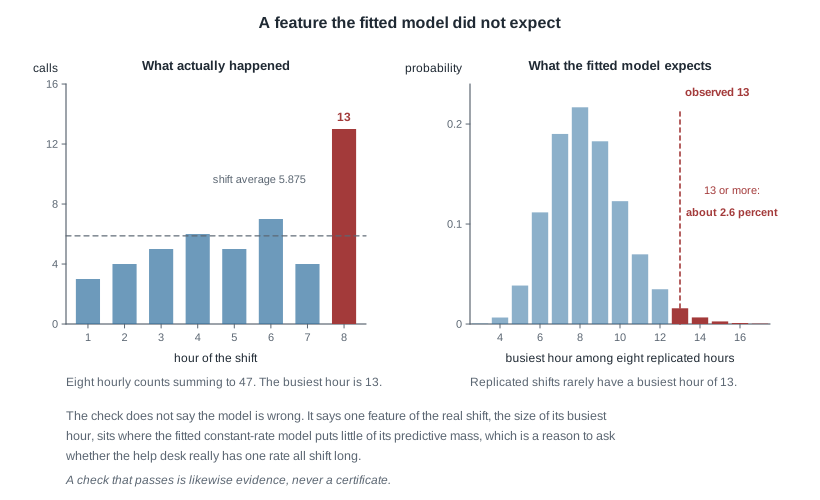
How to say what this means. The real shift’s busiest hour sits where the fitted model puts about 2.6 percent of its predictive mass. That is a flag, not a refutation: a genuinely constant-rate desk can have one hour of 13. What the check does is direct attention at the assumption that should have been suspicious all along: help desks have rush periods, and a model with a single \(\lambda\) for the whole shift cannot represent one.
What follows, and what the check does not settle. The honest report says the estimate of 5.0 calls per hour is a shift average, that the constant-rate assumption is doubtful, and that a plan built on the hour-by-hour predictive interval will understate the busy period. It does not say the model is refuted, and it would not have certified the model had the observed 13 landed in the middle. A passing check tells you only that this feature did not contradict the model. Two honesties belong in the report as well: the replicates were compared against the same eight hours used to fit the model, which makes the check mildly optimistic, and the 2.6 percent moves under a different seed.
The misreading to avoid
Here is the sentence students write, almost word for word, in the week after they meet credible intervals: “There’s a 95 percent chance the next hour has between 3.71 and 6.48 calls.” It is wrong twice over.
The first error is about what the interval describes. The interval 3.711 to 6.478 came from the posterior for \(\lambda\), a rate averaged over the long run, while next hour’s calls are a whole number drawn from a Poisson distribution once \(\lambda\) is fixed. The interval never had anything to say about a single hour, and you can watch it fail: it excludes 3 calls and excludes 7 calls, both perfectly ordinary hours at this desk.
The second is about width. A student who has grasped that the interval is about the rate often still expects the predictive interval to be a slightly stretched version of it. It is not: 1 to 10 against 3.71 to 6.48, standard deviations 2.345 against 0.7071. The commute is starker, 11.75 to 43.94 against 24.21 to 31.48. That gap is neither a defect nor conservatism. It is the sampling variability of one outcome, a property of the world, added to leftover uncertainty about the parameter, a property of your information.
A useful test before writing any interval down: finish the sentence “there is a 95 percent probability that …” out loud. If what follows is a parameter, an average, or a rate, you want the credible interval; if it is something you could go and measure tomorrow, you want the predictive interval. A third confusion, between credible and confidence intervals, is Week 12’s business.
One smaller misreading is worth heading off: “the wider interval means the model is worse.” A wide predictive interval is not a failing model, and one that looks suspiciously narrow beside the scatter in your data is the one to distrust.
Practice on your own
These are for your own checking, not for submission. Use a calculator and R.
A quieter desk. Keep the Gamma(3, 2) prior, but suppose the shift logged 12 calls in 8 hours instead of 47. Find the posterior shape, rate, mean, and standard deviation, then check that the two weights reproduce the posterior mean. Does the prior matter more here, and why?
Doubling the shift. Take a second identical shift, so 94 calls over 16 hours, updated from the original Gamma(3, 2) prior. By what factor does the posterior standard deviation shrink, and by what factor the predictive standard deviation for one new hour? Explain the difference using the variance decomposition.
A tighter prior on the commute. Replace the commuter’s prior standard deviation of 5 minutes with 2 minutes, keeping the prior mean at 30. Recompute the prior and posterior precisions, the posterior mean, and the posterior standard deviation. How far does the posterior mean move, and does the predictive interval for one trip change much?
Choosing the interval. For each, decide whether it needs a credible or a predictive interval and say why: (a) how long is my commute on average; (b) should I leave at 7:35 to arrive by 8:15;
- is the desk’s arrival rate above five calls an hour; (d) how many chairs should be staffed for the coming hour.
Another test quantity. For the shift log 3, 4, 5, 6, 5, 7, 4, 13, let \(T(y)\) be the number of hours with 3 or fewer calls. Compute it for the real data, then write the R that would generate its distribution under the fitted model, predicting first whether it flags the constant-rate assumption as sharply as the busiest hour did.
Where to read more
- This week aligns with Chapter 5 and Chapter 8 of the course’s primary text, Bayes Rules!; both are linked here, Chapter 5 and Chapter 8. Read them alongside this page rather than instead of it.
- The code above uses only base R and the
statspackage that ships with The R Project for Statistical Computing. Ifqnbinomis new, run?qnbinomand read the parameterization note: the negative binomial has two common parameterizations and they are easy to mix up. - Statistical Rethinking is a well-regarded alternative treatment of posterior prediction, named in words here for anyone wanting a second voice on it.
- Course pages: the notes index, the syllabus, the schedule, and the resources page. Availability and licensing for every source in this course are still being confirmed, so treat the course pages as the reliable route.
- Revisit Week 4 for the arithmetic this week generalizes, and Week 5 for a prior strong enough to move a conclusion.
Where this goes next
Week 7 is where the closed forms stop. Every posterior on this page came out in a named family because the prior and likelihood were chosen to make it so, and that will not survive a model with two or three parameters or a prior that is not conjugate. Next week you will approximate this same help desk posterior on a grid and then with Markov chain Monte Carlo, checking both against the exact Gamma(50, 10) derived here. The diagnostics that come with simulation are that week’s real content, and the line drawn here applies there too: a clean diagnostic says the algorithm did not obviously fail, not that the model is right.
The posterior predictive idea has a longer road ahead of it. Choosing a test quantity and asking where the real data fall among replicates becomes a systematic part of model checking for regression in Week 11, and the predictive distribution becomes the object a decision is made on in Week 14. Carry one sentence forward: a distribution for a parameter and one for a future observation are different objects with different widths, and confusing them turns a correct posterior into a wrong recommendation. The course home page lays out all fifteen weeks in order.