Week 1 — Bayesian thinking and uncertainty
Where this week starts
Your previous statistics course taught you to turn data into an estimate and attach a standard error, a confidence interval, or a p-value to it. All of that machinery answers a question about the procedure: if the world stayed the same and you repeated the study many times, how would the numbers you computed behave?
That is a real question, but rarely the one that brought you to the data. A plant manager who has just inspected forty bottles wants to know how likely it is that this capping machine, the one bolted to the floor in front of her, is leaving loose caps at a rate she cannot live with. That is a statement about a fixed, unknown quantity, and the classical toolkit deliberately refuses to make it, because it reserves probability for things that vary.
This week is about the other choice: use probability to describe what you do not know, then let data change that description. Before the data arrive you write down what is plausible; the data speak through a likelihood; what comes out is again a distribution, not a number, and every summary you might want is read off it afterward. There is no calculus on this page and almost no algebra, only arithmetic, and you should do it as you read.
Why this matters outside the classroom
A small bottling line has just refitted its capping head. A loose cap means a returned case, and the maintenance crew must decide tonight whether to pull the head for another adjustment. They inspect forty bottles and find four loose caps. One in ten sounds alarming. But forty bottles is a small inspection, the crew has installed dozens of these heads and has usually seen them settle at one in twenty or below, which makes a higher rate unlikely rather than impossible, and “one in ten” is a lone number carrying no sense of how firmly the data hold it.
The Bayesian version of that meeting produces a distribution over the possible rates, built from what the crew knew plus what the forty bottles said, from which you read the chance that the rate is at least one in ten and hand it to whoever owns the decision. It does not make the decision, and it does not make the machine good or bad; it reports the state of the evidence in a form someone can act on.
What you will be able to do
- Classify a quantity as one that varies from repetition to repetition or one that is fixed but unknown, and say which kind of uncertainty it carries.
- State the two readings of probability, long-run frequency and degree of belief, and give a claim only one of them can express.
- Compute a posterior by hand across a short list of candidate values, naming the prior, likelihood, and posterior as you go: multiply, total, divide.
- Read a mean, an interval, or a threshold probability off a posterior, and say what it does and does not license.
- Explain why a stated prior is an inspectable assumption, and describe the check that catches a prior which ruled out the truth.
Terms and notation worth fixing
These symbols mean the same thing in every unit of this course.
| Symbol | What it means here |
|---|---|
| \(\pi\) | a probability or proportion parameter: this week, a machine’s long-run loose-cap rate |
| \(\theta\) | a generic unknown parameter, when the specific letter does not matter |
| \(y\) | the data you observed; \(n\) is how many observations there are |
| \(\tilde y\) | a new outcome the model predicts but you have not yet seen |
| \(p(\theta)\) | the prior: your description of the unknown before these data |
| \(p(y \mid \theta)\) | the likelihood: how plausible the observed data are under each parameter value |
| \(p(\theta \mid y)\) | the posterior: your description of the unknown after these data |
| \(p(y)\) | the prior predictive distribution of data, which also serves as the normalizing constant |
| \(\propto\) | “is proportional to”: equal after dropping factors free of the parameter |
Read \(p(\theta \mid y)\) aloud as “the distribution of the unknown parameter given the data we observed”: the bar is the word “given”, and everything right of it is held fixed.
Two kinds of not knowing
Most confusion in a first Bayesian course traces to one distinction nobody states carefully, so it gets stated carefully here: there are two very different reasons a number can be uncertain, and probability is used for both.
What varies and what is merely unknown
Some quantities genuinely change from one instance to the next. How many of forty inspected bottles carry a loose cap is one: inspect forty more tomorrow and the count differs, maybe one, maybe five. That variation is a physical fact about the process. If the rate really were 0.05, the count follows a binomial distribution, and a count of two would have probability 0.278, a count of six 0.010.
Other quantities do not vary at all. The machine’s loose-cap rate is a single number, fixed the moment the head was bolted down; inspect every bottle the line will ever produce and you would know it exactly. It is uncertain only because you have not seen enough to pin it down: that is uncertainty about the world, not variation in it.
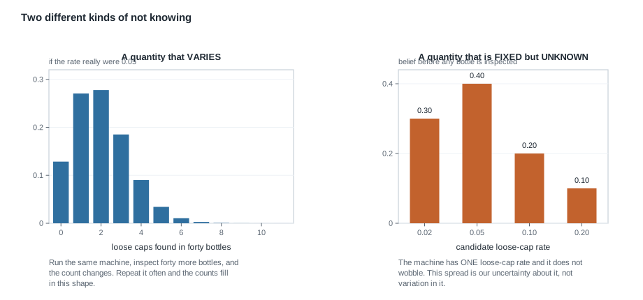
Both panels are drawn as probability, but they answer different questions. On the left the axis is an outcome you could observe and the heights are frequencies the world would produce; on the right the axis is a parameter you can never observe directly and the heights are weights you assign. Classical statistics is comfortable with the left panel and declines to draw the right one.
Two readings of probability, and why the course keeps both
Behind that distinction sits an unsettled question about what “probability” means, and you should be able to state both standard readings fairly. The long-run frequency reading says a probability is the share of times an outcome occurs in a long sequence of repetitions: a fair coin has probability one half of landing heads because, flipped enough times, the running share settles near one half. The degree of belief reading says a probability measures how strongly a claim is supported by what you currently know, which makes it sensible to say there is about a 55 percent chance that this machine’s rate is at least one in ten, even though the machine is installed once and there is no long run to count.
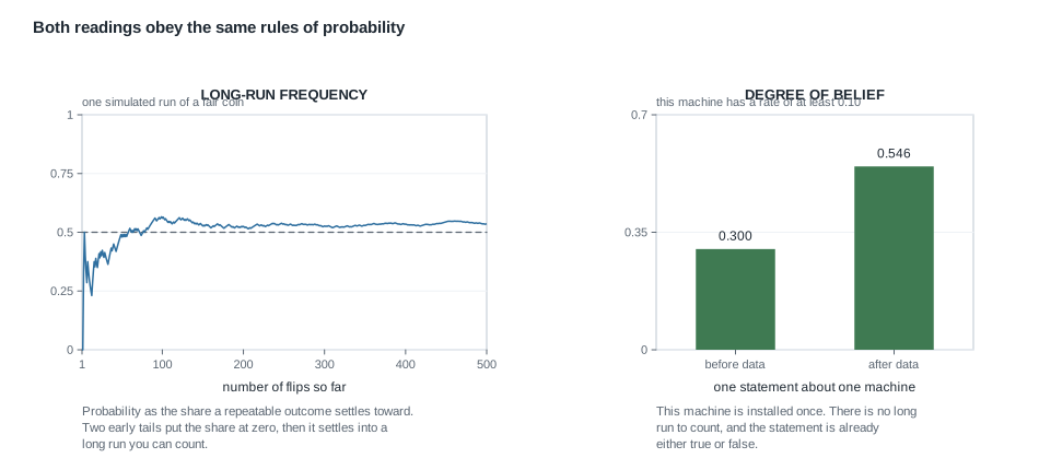
The left panel is one simulated run of five hundred fair flips: the first two came up tails, so the share starts at zero, swings widely, then settles near one half. The right is a claim about a machine that will never be repeated, whose probability rose from 0.300 before the inspection to 0.546 after. Both are probabilities; only the left has a long run you could count.
Be clear on the course’s position. Both readings satisfy the same axioms, and conditional probability behaves identically under either, which is why Bayes’ rule is a theorem nobody disputes. Working statisticians use both. This is not a course arguing that the frequency reading is wrong; it is a course in what becomes sayable once you allow the second, and in the discipline that allowing it demands.
The three parts of every analysis in this course
Every analysis this semester, from next week’s screening test to Week 13’s hierarchical model, has the same three parts. Learn the shape now, while nothing else is in the way.
Prior, likelihood, posterior in one sentence each
The prior, \(p(\theta)\), is a distribution over the unknown saying what you consider plausible before these data. It is not a guess at the value but a range of values with weights on them, written down and reported.
The likelihood, \(p(y \mid \theta)\), runs from the parameter to the data. For each candidate value it asks: if the world were like that, how plausible would the data I actually saw have been? Notice the direction: the data are held fixed at what you observed while the parameter sweeps across candidates. Students almost always read it the other way at first, and Week 3 walks that back.
The posterior, \(p(\theta \mid y)\), is what you get by combining them: multiply prior weight by likelihood at each candidate, then divide every product by their total so the weights add to one. That is the entire operation, and it is the only formula you need this week.
\[p(\theta \mid y) \;\propto\; p(\theta) \; p(y \mid \theta)\]
The proportionality sign does real work: the products need not add to one, because dividing by their total is what turns relative weights into probabilities, and anything multiplying all candidates equally, such as the \(\binom{n}{y}\) in a binomial likelihood, cancels in that division.
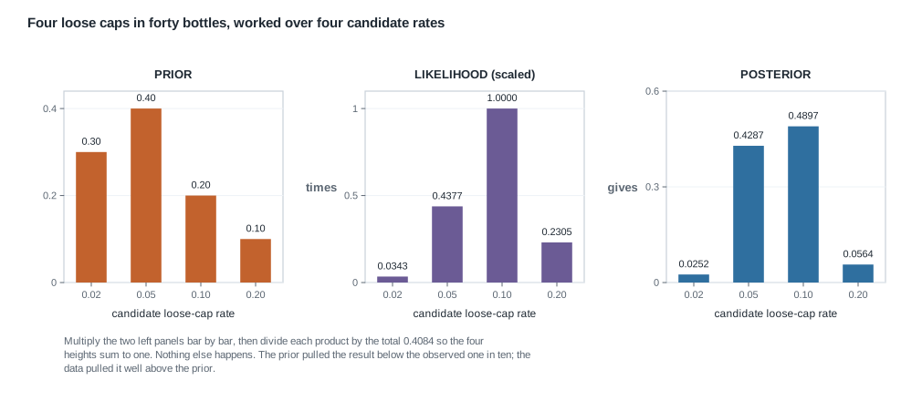
Compare the first and third panels. The prior put most weight on the two smallest rates; the likelihood from four loose caps in forty bottles peaks at 0.10; the posterior lands between them, with 0.05 and 0.10 sharing almost 92 percent of the weight. It is neither the prior nor the data, but what the two together support.
Why the result is a whole distribution
Previously the output of an analysis was a number with a margin of error stapled to it. Here it is a distribution, which is what permits direct probability statements about the unknown. Once you hold a posterior you can ask it anything: which value carries most weight, what the mean is, which range holds 95 percent of the weight, what the probability is that the rate is at least one in ten. Each is a summary read off the same object, and none is the object. Nor is four candidates special; that was a teaching choice so the arithmetic fits on a page.
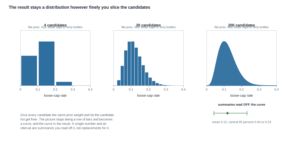
Here every candidate starts with equal prior weight, so the shape is the likelihood’s alone, and the list is refined from four values to twenty to two hundred. The bars narrow and the outline becomes a curve. Week 3 lets the list become a continuum, at which point the curve is a density and the sums become integrals; nothing conceptual changes there.
The interval under the finest panel is the point of the section: on that grid the posterior mean sits at 0.12 and the central 95 percent of the weight runs from about 0.04 to about 0.23. Report those summaries, but read them off the curve rather than substituting them for it.
Worked example — the capping machine’s first forty bottles
Here is the complete arithmetic, with nothing hidden. Work it with a calculator as you read.
The situation. The refitted capping head leaves an unknown long-run share \(\pi\) of bottles with a loose cap. It is one fixed number, and the crew does not know it.
The prior. The crew has installed this model of head many times and will work with four candidate rates and weights on them:
| Candidate rate \(\pi\) | 0.02 | 0.05 | 0.10 | 0.20 |
|---|---|---|---|---|
| Prior weight \(p(\pi)\) | 0.30 | 0.40 | 0.20 | 0.10 |
The four weights add to one, which makes them a distribution. Their implied average rate is \(0.30 \times 0.02 + 0.40 \times 0.05 + 0.20 \times 0.10 + 0.10 \times 0.20 = 0.066\): the crew’s stated position is that the head probably runs near one loose cap in twenty, with a tail out to one in five.
The data. They inspect \(n = 40\) bottles and find \(y = 4\) loose caps: an observed share of \(4/40 = 0.10\).
Step one, the likelihood. Under a candidate rate \(\pi\), the chance of exactly four loose caps in forty bottles is \(\binom{40}{4} \pi^4 (1-\pi)^{36}\), which evaluates to 0.007066, 0.090122, 0.205887 and 0.047452. Only relative size matters, so divide all four by the largest, 0.205887:
| Candidate rate \(\pi\) | 0.02 | 0.05 | 0.10 | 0.20 |
|---|---|---|---|---|
| Scaled likelihood | 0.0343 | 0.4377 | 1.0000 | 0.2305 |
Read that row as a ranking of explanations: 0.10 explains four in forty best, since four in forty is one in ten, while 0.05 explains them about 44 percent as well and 0.02 about 3 percent.
Step two, multiply candidate by candidate.
\[\begin{aligned} 0.30 \times 0.0343 &= 0.01030 \\ 0.40 \times 0.4377 &= 0.17509 \\ 0.20 \times 1.0000 &= 0.20000 \\ 0.10 \times 0.2305 &= 0.02305 \end{aligned}\]
Step three, total and divide. The products total \(0.01030 + 0.17509 + 0.20000 + 0.02305 = 0.4084\), and dividing each by that total gives the posterior:
| Candidate rate \(\pi\) | 0.02 | 0.05 | 0.10 | 0.20 |
|---|---|---|---|---|
| Posterior \(p(\pi \mid y)\) | 0.0252 | 0.4287 | 0.4897 | 0.0564 |
Check one yourself: \(0.01030 / 0.4084 = 0.0252\), and the four weights add to 1.0000. One honest note: because the likelihoods were scaled, 0.4084 is not \(p(y)\) itself but \(p(y)\) divided by the largest of the four likelihoods. The division does not care, which is what \(\propto\) promised.
What the posterior says. Its average rate is \(0.0252 \times 0.02 + 0.4287 \times 0.05 + 0.4897 \times 0.10 + 0.0564 \times 0.20 = 0.0822\), which lands between the prior average of 0.066 and the observed 0.10, a little short of halfway and so still on the prior’s side of the midpoint 0.083. That is what these ingredients should give: the prior put 70 percent of its weight on the two rates below one in ten, and forty bottles is not enough evidence to overturn that. The probability that the rate is at least one in ten is \(0.4897 + 0.0564 = 0.5461\), up from \(0.20 + 0.10 = 0.30\). The worst candidate was demoted, not refuted: 0.20 fell from 0.10 to 0.0564.
What this licenses. One sentence: under these candidates and these prior weights, the evidence puts a little over half the posterior weight on a rate of at least one in ten. It does not license “the rate is 0.0822”, nor “the machine is defective”, a decision needing a cost and a threshold no posterior supplies. Nor does it certify the four-candidate model: 0.07 was never on the table, and a posterior cannot inform you about a value you refused to consider.
The same reasoning, transferred
Change the story completely and the machinery does not move. A coin has been bent and you want the probability \(\pi\) of heads. Take three candidates, 0.3, 0.5 and 0.7, with prior weights 0.25, 0.50 and 0.25, because the bend probably did something but you doubt it did much. Flip it \(n = 12\) times and get \(y = 9\) heads.
The likelihood \(\binom{12}{9} \pi^9 (1-\pi)^3\), scaled by its largest value, is 0.006196, 0.224075 and 1.000000. Multiplying by the priors gives 0.001549, 0.112038 and 0.250000, totalling 0.363587. Dividing through, the posterior is 0.0043, 0.3081 and 0.6876, with average \(0.0043 \times 0.3 + 0.3081 \times 0.5 + 0.6876 \times 0.7 = 0.6367\).
What stayed the same: a fixed but unknown parameter, a stated prior over candidates, a binomial likelihood with the data held fixed, a normalized product. What changed: the subject, the candidate list, the sample size, and a symmetric rather than low-tilted prior. The recipe never noticed, and that portability is why the next eleven weeks are possible.
Second worked example — a prior that ruled out the truth
The first example was a clean application. This one is a failure, and the more instructive, because it shows the check you have to run and what happens when nobody runs it.
The situation. A month later a different technician inspects the same line. The vendor’s service sheet says this model of head “cannot run above one loose cap in ten”, and the technician takes it literally, giving the candidate 0.20 no weight at all:
| Candidate rate \(\pi\) | 0.02 | 0.05 | 0.10 | 0.20 |
|---|---|---|---|---|
| Restricted prior | 0.35 | 0.45 | 0.20 | 0.00 |
The data. A fresh inspection of forty bottles turns up nine loose caps, a share of \(9/40 = 0.225\).
The update. The likelihood \(\binom{40}{9} \pi^9 (1-\pi)^{31}\), scaled by its largest value, is 0.000001, 0.000785, 0.075242 and 1.000000. Multiplying by the restricted prior gives 0.0000002, 0.0003534, 0.0150483 and 0.0000000, totalling 0.0154020. Normalizing leaves essentially 0 on 0.02, 0.0229 on 0.05, 0.9770 on 0.10, and exactly zero on 0.20, with an average rate of 0.0989.
Sit with that, because it looks excellent: over 97 percent of the weight on one candidate, reading as a confident conclusion. It is also badly wrong, and no further data can rescue it. Zero times any likelihood is zero, so a candidate given no prior weight can never gain any, however loudly the data argue.
The same data without the restriction. Run the identical nine-in-forty data through the crew’s original prior. The products are 0.0000002, 0.0003142, 0.0150483 and 0.1000000, totalling 0.1153627, and the posterior is 0.0000, 0.0027, 0.1304 and 0.8668, average rate 0.1865. Same data, same likelihood, and the two analyses disagree about which candidate is most plausible.
The check that should have been run. Before seeing data, ask what data the prior expects: for each count \(\tilde y\) from zero to forty, mix the binomial probabilities across candidates, as \(p(\tilde y = k) = \sum_j p(\pi_j) \binom{40}{k} \pi_j^{\,k} (1-\pi_j)^{40-k}\). That is the prior predictive distribution, and it is where a prior meets reality before any posterior exists.
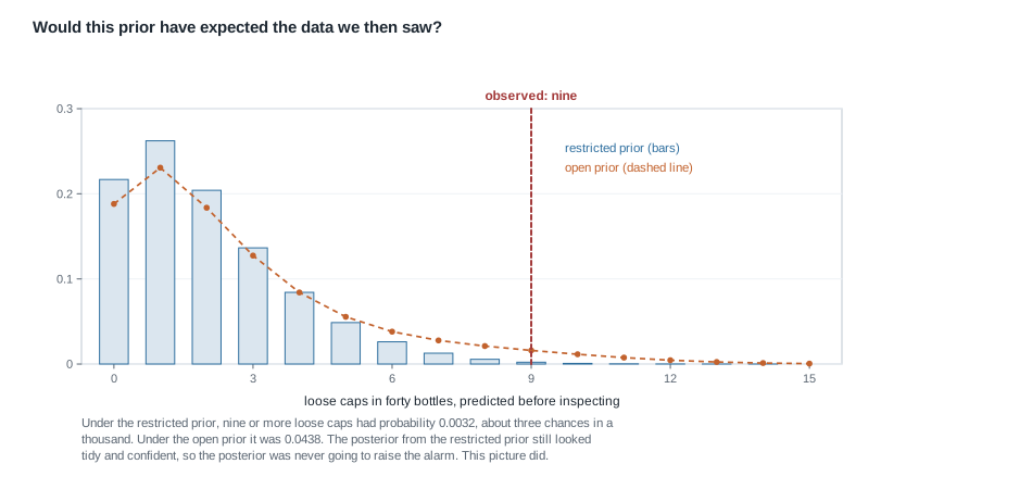
Under the restricted prior the expected count is 1.98 loose caps in forty bottles, and nine or more has probability 0.0032, about three chances in a thousand; under the open prior that tail has probability 0.0438. Neither prior thought nine likely, but one thought it nearly impossible. When the data you collected sit in the far tail of what your model expected beforehand, the model, prior included, falls under suspicion.
What to take from this. The failure was not that the prior was informative; informative priors are fine and often necessary. It was a prior assigning zero to a live possibility, unexamined. A tidy posterior is not evidence that a model is adequate: it summarizes what the model concluded, and a model that has ruled something out will conclude confidently and wrongly without complaining.
The misreading to avoid
Here is the objection as students actually raise it, often with some heat: “Bayesian statistics is just statistics with an opinion mixed in. Pick a prior that leans the way you want and you can get whatever result you like. That is not science.”
Take it seriously, because half of it is correct. The prior does affect the result, and this week’s second example proved it harshly: identical data, two priors, an average moving from 0.0989 to 0.1865. Three things make the objection collapse anyway.
First, the prior is stated. It is written down and available to anyone who wants to disagree. A reader who thinks 0.30, 0.40, 0.20, 0.10 was too optimistic can name the weights they prefer, rerun the arithmetic, and show what changes: an argument that can be had. An analysis that never mentions a prior has not avoided assumptions; it has made them about which model to fit, which observations to exclude, and which test to report, and left every one off the page.
Second, the prior can be checked and varied. The prior predictive check above is a real test, run before any posterior exists, and the restricted prior failed it. Nor should reporting stop at one prior: Week 5 runs four through one data set and reports the range of conclusions as the result. An analysis stable across every defensible prior says the data are decisive; one that is not says something equally important that a single number would hide.
Third, the data win, and you can watch them win. In the first worked example the prior average 0.066 became a posterior average of 0.0822, pulled almost halfway to the observed 0.10 by only forty bottles, and multiplying the data by ten shrinks the prior’s influence toward nothing. A prior is a starting position, not a veto, unless you write it as one by assigning zero.
Two smaller misreadings are worth naming. A posterior probability is not a p-value: 0.5461 is the probability that this machine’s rate is at least one in ten given this model and this prior. And a posterior is not a verdict; deciding what to do about a rate of 0.0822 needs a threshold and a cost that live outside the statistics.
Working reproducibly from day one
This page’s arithmetic fits on a page; almost nothing else this semester will, so the course teaches its computing rather than assuming it. Set the three tools up now, render one small document, and take on the habits below.
Installing R, VS Code, and Quarto
Install them in this order, because each one looks for the one before it. The R Project for Statistical Computing supplies the language and the statistical functions every later week calls. Visual Studio Code is the editor we write in; once it opens, add its R and Quarto extensions from the extensions panel. Quarto is the document system that lets prose, code, and figures live in one file that regenerates itself. Then run quarto check in a terminal: it reports what it found, including whether it located R.
If it reports that R cannot be found, your first render will fail, so settle it now. Any one of these three fixes is enough:
- Put R’s
bindirectory on your PATH. Find the folder inside your R installation that holds the R program itself, add that folder to the PATH environment variable, and open a new terminal so the change takes effect. - Set the
QUARTO_Renvironment variable to the R program itself, not to the folder holding it. Quarto consults that variable before searching anywhere else, so it also settles which of two installed versions gets used. - Render from a shell whose PATH already has R. If typing
R --versionthere prints a version, Quarto started from that same terminal will find R too.
Your first Quarto document
A Quarto document is a plain text file ending in .qmd: a short header fenced by three hyphens above and below, then prose, then code chunks. A chunk opens with a line of three backticks immediately followed by {r} in braces and closes with a line of three backticks. A minimal file starts like this:
---
title: "Week 1 notes"
format: html
---

The crew inspected forty bottles and found four loose caps.
Under that prose goes one chunk. Here is the first worked example as its body, written as a record of what was done rather than output to trust on sight:
# Four candidate loose-cap rates, and the crew's prior weights.
rates <- c(0.02, 0.05, 0.10, 0.20)
prior <- c(0.30, 0.40, 0.20, 0.10)

# Likelihood of 4 loose caps in 40 bottles at each candidate rate.
lik <- dbinom(4, size = 40, prob = rates)

# Multiply, total, divide: the entire update.
posterior <- prior * lik / sum(prior * lik)

round(posterior, 4)             # posterior weights on the four candidates
sum(posterior * rates)          # posterior average rate
sum(posterior[rates >= 0.10])   # posterior probability of at least one in ten
Seven lines of code, and that is the whole method; lik does not need scaling, since dividing by the total handles any common factor. Render the file with quarto render week-01-notes.qmd, or with the render button in Visual Studio Code, and you get an HTML file beside the .qmd carrying prose, code, and output together. quarto preview re-renders each time you save.
Habits that make the work reproducible
Reproducibility is part of the statistics rather than a courtesy added afterward. A Bayesian result is a conditional statement: given this prior, this likelihood, and these data, here is the posterior. A reader who cannot see the prior cannot evaluate the conclusion, and one who cannot rerun the analysis cannot check the sensitivity you reported. Four habits carry most of that weight.
- Fix a seed with
set.seed(1234)before anything random, so a simulation gives the same draws on your machine tomorrow and on a classmate’s today. - Keep code and prose in one document, rather than computing in a console and pasting numbers into a write-up where a reader cannot see where they came from.
- Re-render from a clean start before you hand work in; a document that renders only inside the session you happen to have open is not reproducible.
- Never write a number you cannot regenerate. If it came from a computation, let the document do that computation.
Install the three tools this week, and get one small document rendering while the arithmetic is still this small.
Practice on your own
These are for your own checking, not for submission. Work them with a calculator against the worked examples.
Sort the quantities. For each, say whether it varies or is fixed but unknown, with one sentence on the uncertainty it carries: the number of customers arriving at a help desk between two and three this afternoon; the long-run average number arriving in an hour; whether one particular seed germinates; the germination rate of the lot it came from.
Redo the update with a flatter prior. Same four candidate rates and the same four loose caps in forty bottles, but give every candidate a prior weight of 0.25. The scaled likelihoods are unchanged at 0.0343, 0.4377, 1.0000 and 0.2305. Compute the products, their total, and the posterior, then say which candidates gained weight and why.
Double the data. Suppose the crew had found eight loose caps in eighty bottles, the same observed share. Using the original prior, evaluate \(\binom{80}{8} \pi^8 (1-\pi)^{72}\) at each candidate, scale by the largest, and update. Does the posterior sit closer to the observed share than before, and why should that have been expected?
Break a prior on purpose, then report carefully. Give the candidate 0.05 a prior weight of zero, spread the rest however you like, and update on four loose caps in forty bottles. What posterior weight does 0.05 end up with, and what would change it? Then, from the first worked example’s posterior, write one sentence a maintenance supervisor could act on and a second naming something that first sentence does not establish.
Where to read more
- Bayes Rules!, this course’s primary text. This week aligns with Chapter 1; the home page is bayesrulesbook.com. Read the chapter after this page, since the second pass through an idea is where it sticks.
- Tools. Setup for R, Visual Studio Code, and Quarto is on this page, under “Working reproducibly from day one”. The resources overview is where the course’s reading links are collected.
- Course pages. The syllabus records how the semester is organized and the standing of every source, the schedule lays out the fifteen weeks, and the notes index lists every unit.
- Named but not linked. Statistical Rethinking is a widely used alternative treatment at a somewhat higher level. Availability and licence confirmation is still open for every source here, so obtain them through the library.
Where this goes next
Week 2 makes the update exact in the one setting where every quantity can be counted: diagnostic testing. You will count how many of a screened population have a condition, how many of them test positive, and how many healthy people also test positive, and find that the share of positive results which are true can be startlingly small even for a test that is right almost every time. That week also introduces the odds form of Bayes’ rule, where sequential updating becomes something you can do in your head. Read it at week-02.qmd once it is posted.
After that the parameter goes continuous. Weeks 3 and 4 replace the short candidate list with a whole interval, using a seed lot’s germination rate as the running case, and this page’s bar charts become the smooth densities you glimpsed in the third figure. Counts, means, regression, model checking, and hierarchical structure follow, but the shape never changes: state what is plausible, let the data speak through a likelihood, look at the distribution that results, and ask whether that model could have produced the data you have. Return to the course home page or the notes index for the map.