Week 10 — Causal diagrams and backdoor reasoning

Confounders, colliders, backdoor paths, adjustment sets, and bad controls

The week question

Last week you saw the tutoring-center study shrink from a naive \(+8.0\)-point gap to an adjusted \(+3.0\) once you stratified on prior ability. That raises a sharper question that this week answers head on: how do you know which variables to adjust for, and which ones it would be a mistake to touch? The tool is a causal diagram — a small picture of your assumptions about what causes what. The week question is therefore: given a diagram of how a study’s variables relate, which variables must you adjust for to read a causal effect, and which would silently bias the answer if you did?

This is a design-reasoning question, not a modeling question. The diagram is decided before any regression runs, and it is the design — what was assigned, what was merely observed, what came before treatment and what came after — that the diagram encodes.

Why this matters

In a randomized experiment, random assignment breaks every backdoor path for you: nothing measured before treatment can be a common cause of treatment and outcome, because treatment was decided by a coin. In an observational study like the tutoring-center study, you have to do that work by reasoning, and the work is easy to get wrong in a way no software will warn you about. Adjusting for the wrong variable does not throw an error. The code runs, the number moves in a plausible-looking direction, and the estimate is now biased.

A causal diagram is the cheapest insurance against that silent failure. It forces you to write down, as arrows, the assumptions you are already relying on, and it then tells you mechanically what to adjust for and — just as importantly — what to leave alone. The single most common observational-study error is a bad control: adjusting for a variable that sits after treatment, which removes part of the very effect you set out to measure. The diagram is what makes that error visible.

The discipline here connects directly to the course’s spine. Random sampling earns population claims; random assignment earns causal claims. When you lack assignment, a diagram plus a defensible adjustment set is the closest an observational study can come to a causal claim — and it only works for confounders you actually measured. That limit is the whole reason the well-designed experiment is worth so much.

Learning goals

By the end of this week you should be able to:

• read a causal diagram as a set of nodes (variables) and directed edges (assumed direct causes), and trace a path and a backdoor path between treatment and outcome;
• classify a third variable by its role — confounder (common cause), mediator (on the causal path), or collider (common effect) — and say what each role implies for adjustment;
• choose an adjustment set of pre-treatment variables that blocks every backdoor path, and explain why it is correct in words, not just by output;
• recognize a bad control (adjusting for a mediator or a collider) and explain the direction of the bias it causes;
• state plainly that a diagram encodes assumptions, not conclusions, and that an unmeasured confounder is a standing limit no adjustment can fix.

Core vocabulary

• Node — a variable in the study (treatment, outcome, or a third variable), drawn as a labelled point.
• Directed edge \(A \to B\) — the assumption that \(A\) is a direct cause of \(B\). Every arrow is a claim you are making, justified by design or domain knowledge, not by the data.
• Path — any route between two nodes along the edges, with or against the arrow directions.
• Causal path — a path from treatment \(Z\) to outcome \(Y\) whose arrows all point forward, \(Z \to \dots \to Y\): this is how the treatment actually moves the outcome.
• Backdoor path — a non-causal route from \(Z\) to \(Y\) that starts with an arrow into \(Z\) (so \(Z \leftarrow \dots \to Y\)). It carries confounding and must be blocked.
• Confounder — a pre-treatment common cause of both \(Z\) and \(Y\) (\(Z \leftarrow C \to Y\)). It opens a backdoor path; you adjust for it to close the path.
• Mediator — a post-treatment variable on the causal path \(Z \to M \to Y\). It carries part of the effect; you do not adjust for it if you want the total effect.
• Collider — a common effect of two variables (\(A \to K \leftarrow B\)). A collider blocks its path by default; adjusting for it opens a spurious association — the opposite of a confounder’s behaviour.
• Adjustment set — a set of pre-treatment variables that blocks every backdoor path, containing no mediators and no colliders.
• Bad control — adjusting for a mediator or a collider; it biases the causal estimate even though the software runs cleanly.

Concept development

Nodes, edges, paths, and the backdoor

A causal diagram is built from nodes (variables) joined by directed edges (arrows). An arrow \(A \to B\) says “I assume \(A\) is a direct cause of \(B\).” There are no undirected edges and no cycles — that is what makes it a directed acyclic graph (DAG). The picture is entirely a statement of your assumptions; it contains no numbers and no results.

A path is any chain of edges connecting two nodes, traced with or against the arrows. Between a treatment \(Z\) and an outcome \(Y\), two kinds of path matter. A causal path runs forward from \(Z\) to \(Y\), like \(Z \to Y\) or \(Z \to M \to Y\); this is the effect you want to measure. A backdoor path is a non-causal route that begins with an arrow pointing into \(Z\) — for example \(Z \leftarrow C \to Y\). A backdoor path lets association flow between \(Z\) and \(Y\) for a reason that has nothing to do with \(Z\) causing \(Y\). That is confounding, and the estimand you care about is recoverable only once every backdoor path is blocked.

The design move here is to separate the route you want to keep open (the causal path) from the routes you must close (the backdoor paths). The diagram is what tells the two apart, because the diagram knows the direction of every arrow.

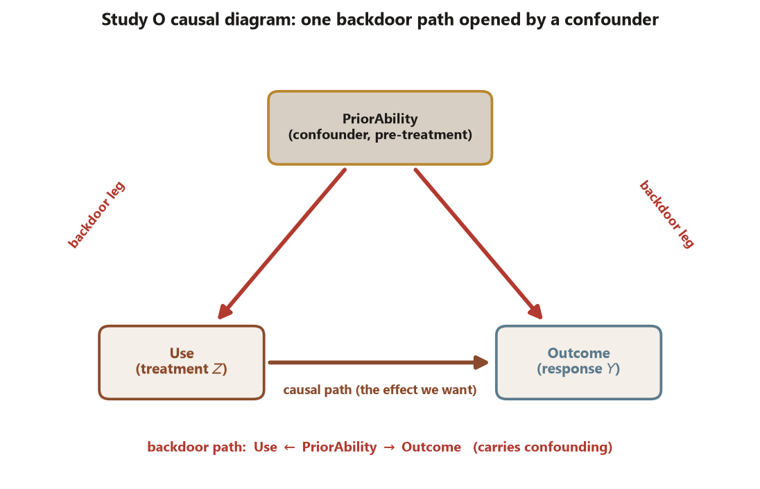
Figure 1: A causal diagram names your assumptions as arrows. This is the assumed diagram for the tutoring-center study. PriorAbility is a pre-treatment confounder: it points into both Use (the treatment \(Z\)) and Outcome (the response \(Y\)), and those two red arrows are the two legs of the backdoor path Use \(\leftarrow\) PriorAbility \(\to\) Outcome that carries confounding. The single brown arrow Use \(\to\) Outcome is the causal path you actually want to measure. Reading a causal effect means keeping that brown path open while blocking every red backdoor. Synthetic; seed 45403.

The three roles a third variable can play

The same third variable can demand opposite handling depending on the role it plays in the diagram. This is the heart of the week, and it is where intuition most often misleads.

• A confounder is a common cause: \(Z \leftarrow C \to Y\). It sits on a backdoor path, so it injects confounding. You adjust for it (stratify, or include it as a covariate) to close that backdoor.
• A mediator is on the causal path, \(Z \to M \to Y\). It is post-treatment — it happens because of the treatment — and it carries part of the effect. If you adjust for a mediator, you subtract off the slice of the effect that travels through it, so the total effect you wanted shrinks toward zero. You do not adjust for a mediator when the total effect is the target.
• A collider is a common effect: \(A \to K \leftarrow B\). By default a collider blocks the path through it, so \(A\) and \(B\) are unassociated through \(K\). But the moment you adjust for the collider, you open a spurious path and manufacture an association between \(A\) and \(B\) that was never there. A collider behaves backwards from a confounder: leaving it alone is correct, adjusting for it is the error.

The rule that falls out of this is simple to state and easy to violate: adjust for confounders, never for mediators or colliders. A confounder is always pre-treatment; a mediator and an adjustment-induced collider bias are post-treatment phenomena. So a fast, robust screen is to ask of every candidate variable: did this happen before treatment, or after? Pre-treatment common causes are fair game; anything post-treatment is suspect.

Adjustment sets, bad controls, and what a diagram cannot buy you

An adjustment set is a set of variables that, when you condition on them, blocks every backdoor path from \(Z\) to \(Y\) while leaving the causal path open. The informal backdoor rule is: list the variables you believe cause the treatment, the outcome, or both; mark each as pre- or post-treatment; find the backdoor paths; and choose a set of pre-treatment variables that blocks all of them — adding nothing post-treatment. A correct adjustment set contains only confounders (or other pre-treatment variables that help block paths), and never a mediator or a collider.

Putting a mediator or a collider into the adjustment set is a bad control. It is the most dangerous error in observational analysis precisely because it is invisible: the regression runs, the coefficient changes, and the change looks like a more careful answer. Adjusting for a mediator removes real signal (it biases the total effect toward zero); adjusting for a collider adds fake signal (it manufactures association). Either way the diagram — not the output — is what would have caught it.

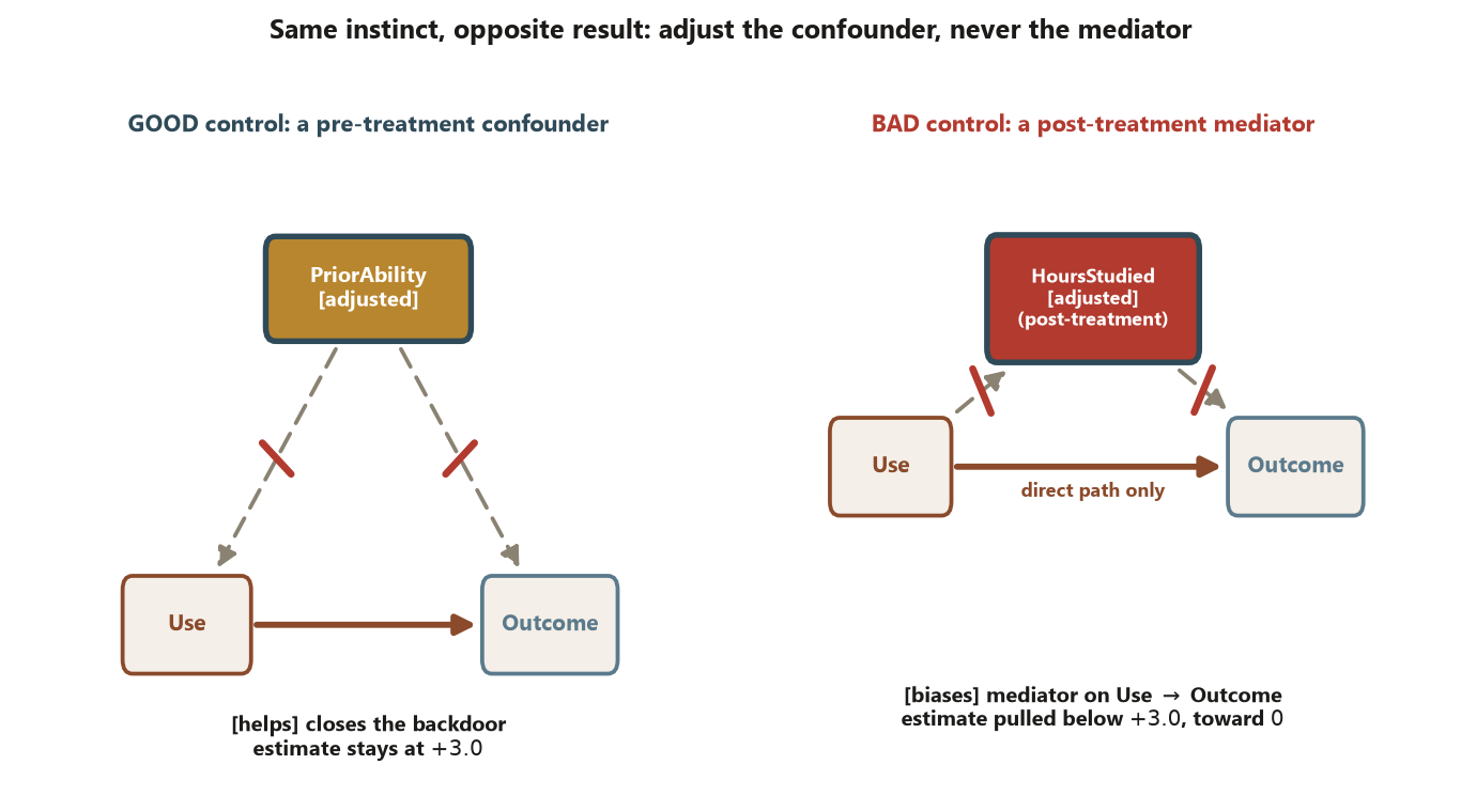
Figure 2: One instinct, opposite consequences. Adjusting for the pre-treatment confounder PriorAbility (left) is a good control: it closes the backdoor while leaving the causal path open, so the estimate stays at the adjusted \(+3.0\). Adjusting for the post-treatment mediator HoursStudied (right) — which sits on the causal path Use \(\to\) HoursStudied \(\to\) Outcome — is a bad control: it strips out the slice of the effect that runs through extra studying and pulls the estimate below \(+3.0\), toward \(0\). The one-question screen is whether the variable is pre- or post-treatment. Synthetic; seed 45403.

Finally, a diagram is honest about its own limits. It does make your assumptions explicit and tell you what to adjust for. It does not prove those assumptions, and it cannot rescue a confounder you never measured: if a real common cause is unmeasured, no adjustment can close its backdoor. That standing limit of observational evidence is exactly why random assignment, which closes all backdoors by design, is worth so much (Risk 15: every arrow you draw — and every one you omit — is a claim the design must support).

Worked examples

Worked example — the tutoring-center DAG (recurring study, locked numbers)

Study O asks whether using the tutoring center improves an end-of-term performance score. Students chose whether to use the center — there is no random assignment — so this is observational, and any causal reading has to survive the backdoor reasoning. The recurring counts and effects are fixed: users \(n = 120\), non-users \(n = 180\) (total \(300\)); the naive mean difference is users \(82.0\) minus non-users \(74.0 = +8.0\); stratifying on the pre-treatment prior-ability tier yields the adjusted \(+3.0\), so confounding inflated the naive estimate by \(+5.0\).

Author the diagram as accessible text (a node-and-edge list plus prose), not an image. The assumed diagram:

Nodes. Use (treatment \(Z\) — used the tutoring center, yes/no), Outcome (response \(Y\) — end-of-term score), PriorAbility (a pre-treatment covariate — preparation/motivation before the term), and HoursStudied (hours studied during the term).

Edges.

• PriorAbility -> Use — more-prepared, more-motivated students are likelier to choose the center.
• PriorAbility -> Outcome — more-prepared students score higher anyway, regardless of the center.
• Use -> Outcome — the causal effect we want to estimate.
• Use -> HoursStudied -> Outcome — using the center leads to more studying, which lifts the score.

Reading the diagram.

• The path Use <- PriorAbility -> Outcome is a backdoor path: it starts with an arrow into Use, so PriorAbility is a confounder. It is pre-treatment, it causes both Use and Outcome, and it must be adjusted for. Closing this backdoor is exactly what drops the naive \(+8.0\) to the adjusted \(+3.0\).
• HoursStudied lies on the causal path Use -> HoursStudied -> Outcome, so it is a mediator — it is post-treatment (a consequence of using the center). Adjusting for it would be a bad control: it would strip out the part of the effect that runs through extra studying and bias the estimate downward.

So the correct adjustment set is \(\{\text{PriorAbility}\}\) — and emphatically not \(\{\text{PriorAbility}, \text{HoursStudied}\}\). The first closes the backdoor and leaves the causal path intact; the second closes the backdoor but also amputates part of the effect. The diagram, not the regression output, is what tells you which is which (Risk 4, Risk 7).

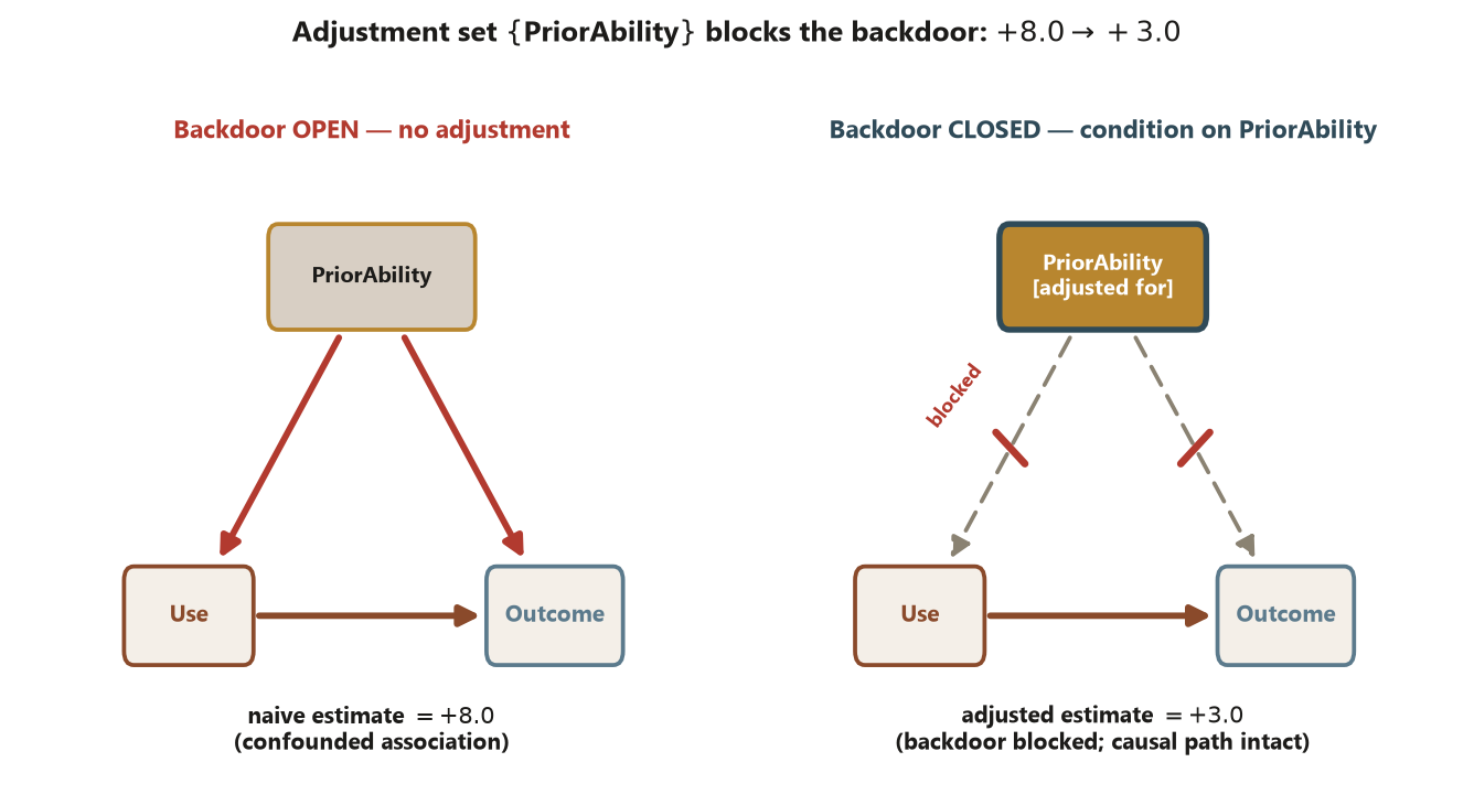
Figure 3: Adjusting for the one confounder closes the backdoor. On the left the backdoor is open and the unadjusted contrast is the naive \(+8.0\) — a confounded association, because stronger students both use the center and score higher. Conditioning on the pre-treatment confounder PriorAbility (right) blocks both backdoor legs while leaving the causal path Use \(\to\) Outcome untouched, dropping the estimate to the adjusted \(+3.0\). That \(+8.0 \to +3.0\) shrinkage is the backdoor closing. Synthetic; seed 45403.

The static R below generates data from this diagram and shows the naive versus adjusted contrast, plus what a bad control does. It is shown as teaching, not executed in this diagnostic.

# Study O — tutoring-center DAG: data generated FROM the assumed diagram.
# Synthetic; seed set. Static, non-executed code (shown as teaching).
set.seed(45403)

n <- 300                                  # 300 students (the locked Study O size)

# PriorAbility: a PRE-treatment confounder (cause of BOTH Use and Outcome).
prior <- rnorm(n, mean = 0, sd = 1)

# Use: more-prepared students are likelier to use the center  (PriorAbility -> Use).
#   Calibrated to the locked slice: intercept -0.54 puts the use rate near 40%
#   (E[users] = 120 of 300; this seed gives 114/186), and slope 1.34 makes the
#   users sit a full 1.0 SD above non-users in prior ability.
use   <- rbinom(n, size = 1, prob = plogis(-0.54 + 1.34 * prior))

# HoursStudied: POST-treatment mediator on Use -> HoursStudied -> Outcome.
hours <- 0.8 * use + 0.5 * prior + rnorm(n)

# Outcome: PriorAbility -> Outcome (backdoor) + DIRECT Use effect 2.2
#          + indirect via hours (0.8 * 1.0 ~ 0.8) = total true Use -> Outcome effect ~ +3.0.
#   Reduced form: 76 + 3.0*use + 5.0*prior — with the 1.0-SD prior gap this puts the
#   naive contrast at the locked +8.0 and the group means near the locked 82.0 / 74.0.
outcome <- 76 + 2.2 * use + 4.5 * prior + 1.0 * hours + rnorm(n)

# NAIVE difference (no adjustment): leaves the backdoor OPEN.
naive    <- coef(lm(outcome ~ use))["use"]              # ~ +8.0  (this seed: +8.27; confounded)

# ADJUSTED for the confounder only: closes the backdoor. Correct adjustment set.
adjusted <- coef(lm(outcome ~ use + prior))["use"]      # ~ +3.0  (this seed: +2.80; recovers the effect)

# BAD CONTROL: also adjusting for the post-treatment mediator HoursStudied.
badctrl  <- coef(lm(outcome ~ use + prior + hours))["use"]  # targets the DIRECT 2.2, not the total
                                                            # (this seed: +2.00 — mediator/bad-control bias)

Interpretation. The naive coefficient is about \(+8.0\) because the backdoor through PriorAbility is open — that number conflates the center’s effect with the fact that stronger students both use the center and score higher, so it is an association, not a causal effect. Adjusting for the confounder PriorAbility closes the backdoor and recovers about \(+3.0\), the design move being: stratify on a pre-treatment common cause to block the backdoor path. The bad-control fit, which also conditions on the post-treatment mediator HoursStudied, pulls the estimate below \(+3.0\) — a biased number that looks careful but answers the wrong question. The claim the adjusted analysis supports is a causal effect of about \(+3.0\) only if prior ability is the sole confounder and it is measured well; it is not a guarantee, because an unmeasured confounder would leave a backdoor open (Risk 15).

Note the intended parallel with Study E: the adjusted observational \(+3.0\) deliberately matches the experiment’s randomized \(d = 3.0\). Careful adjustment approximates what random assignment guarantees — but only when the confounder is measured and the diagram is right.

Worked example — exercise, health, and a fitness-tracker collider (transfer)

Now move to a new context to see the collider role, which the tutoring-center study does not contain. A researcher asks whether regular exercise (\(Z\)) improves a cardiovascular-health score (\(Y\)) among adults. The numbers here are illustrative and clearly distinct from the locked study slice.

Nodes. Exercise (treatment \(Z\)), Health (outcome \(Y\)), Age (a pre-treatment covariate), and OwnsTracker (whether the person bought a fitness tracker).

Edges.

• Age -> Exercise and Age -> Health — older adults exercise less and have lower scores, so Age is a confounder on the backdoor Exercise <- Age -> Health.
• Exercise -> Health — the causal effect we want.
• Exercise -> OwnsTracker and Health -> OwnsTracker — active people buy trackers, and health-conscious people buy trackers. So OwnsTracker is a common effect of both Exercise and Health: it is a collider (\(Exercise \to OwnsTracker \leftarrow Health\)).

Reading the diagram. The adjustment set is \(\{\text{Age}\}\): Age is the only confounder, and closing its backdoor is the whole job. OwnsTracker must be left out. By default the collider blocks its own path, so exercise and health are not linked through tracker ownership. But if you condition on tracker owners — say you analyze only people who bought a tracker — you open the collider path and manufacture a spurious negative association: among tracker owners, someone who exercises a lot can have ended up with a tracker for that reason alone, so they need not be especially healthy, making exercise look falsely unhelpful.

Suppose the unadjusted exercise–health difference is \(+6\) points, the age-adjusted (correct) effect is \(+4\) points, but the tracker-owners-only “collider-conditioned” estimate comes out near \(+1\). The design reading is that \(+4\) is the defensible estimate — it closes the age backdoor and touches no post-treatment or collider variable — while the \(+1\) is a bad control artifact created by selecting on a common effect (Risk 4). The claim this study supports is that exercise is associated with about \(+4\) points of better health adjusting for age, and is causal only under the assumption that age is the sole confounder; selecting on the tracker would corrupt even that (Risk 7, Risk 15).

A common mistake

The signature mistake this week is the bad control: throwing a variable into the adjustment set because it “seems related to the outcome,” without asking whether it came before or after treatment. More variables feel safer — but a mediator or a collider in the adjustment set makes the answer worse, not better, and nothing in the output flags it.

Two flavours, both shown above. Adjusting for a mediator (like HoursStudied in the tutoring study) removes part of the real effect, biasing the total effect toward zero — you have measured a “direct effect holding studying fixed,” which is not the question you asked. Adjusting for a collider (like OwnsTracker, or, equivalently, restricting the sample to tracker owners) opens a path and manufactures an association that does not exist. The fix is one disciplined screen: every variable in the adjustment set must be pre-treatment and must block a real backdoor path. Do not adjust reflexively; adjust to close a specific backdoor, and justify each arrow you drew. A diagram with an arrow you cannot defend is worse than no diagram, because each edge — and each omission — is a causal claim the design must support (Risk 4, Risk 7, Risk 15).

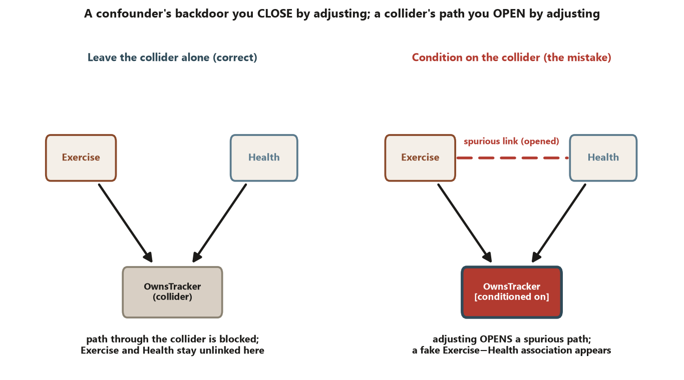
Figure 4: With a collider, adjusting does the opposite of what you expect. A collider is a common effect: here both Exercise and Health cause OwnsTracker. On the left, leaving the collider alone keeps its path blocked, so Exercise and Health stay unlinked through it. On the right, conditioning on the collider — for example, analyzing only tracker owners — opens a spurious path and manufactures a fake Exercise–Health association that was never there. A confounder’s backdoor you close by adjusting; a collider’s path you open by adjusting — the exact reversal that makes reflexive adjustment dangerous. Synthetic; illustrative.

Low-stakes self-checks (ungraded)

These are for your own practice — ungraded, no submission.

1. In the tutoring-center DAG, trace the backdoor path from Use to Outcome in words, and name the single variable whose adjustment closes it. Which locked number is the open-backdoor estimate, and which is the closed-backdoor estimate?
2. A classmate adds HoursStudied to the adjustment set “to be thorough.” Name the role HoursStudied plays, say whether it is pre- or post-treatment, and predict the direction the estimate moves.
3. In the exercise example, explain in one sentence why adjusting for Age is required but adjusting for OwnsTracker is forbidden — using the words confounder and collider.
4. True or false: a small p-value on the adjusted coefficient proves the adjustment set was correct. Explain what a p-value can and cannot tell you about the design (Risk 5).
5. Write down one variable you would need to measure for the tutoring-center causal claim to be credible, and state what happens to the backdoor if it stays unmeasured.

Reading and source pointer

This week is grounded in the instructor notes (primary), which set the first-course, applied level of the causal-diagram material: nodes and edges, paths and backdoor paths, the three roles of a third variable, the adjustment set, and the bad-control trap. Causal Inference: What If (Hernán & Robins) is named only as an optional advanced reference that calibrates the vocabulary and level — it is freely readable online but is linked and cited only, with no content reproduced here. The companion adjustment-by-simulation lab draws on the ModernDive simulation workflow for its reproducible R posture.

These notes are the course’s own synthesis, grounded in but not copied from the sources.

Public vs. graded

These notes, the examples, and the practice here are public and ungraded — study material only. No graded prompts, answer keys, rubrics, point values, or due dates appear on this site. Graded design checkpoints, weekly quizzes, design memos and homework, applied design labs, the midterm, the final design project, and the final exam live in Blackboard (the LMS), which is authoritative for due dates, submissions, and grades. If this page and Blackboard ever disagree, follow Blackboard.

Looking ahead

Next week the course pivots from causal evidence to sampling. Week 11 takes up surveys and sampling frames with Study S — the campus study-habits survey — where the central distinction is no longer assignment but random sampling: a target population of \(12{,}000\) undergraduates, a registrar frame of \(11{,}400\) (a coverage gap), an SRS giving \(\hat p = 0.45\), and a nonresponse bound that dwarfs the sampling interval. The backdoor reasoning you built this week earns causal claims; sampling, which we turn to next, earns population claims — and they are not interchangeable.

See also

• Week 9 — Observational studies — the naive \(+8.0 \to\) adjusted \(+3.0\) shrinkage this week diagrams.
• Week 11 — Surveys and sampling frames — from causal claims to population claims.
• Lab 10 — Confounding and adjustment by simulation — generate data from a DAG and watch adjustment recover the effect (and a bad control break it).
• Causal-diagram guide — the standalone reference for drawing and reading DAGs.
• Design glossary — confounder, mediator, collider, adjustment set, bad control.
• Design reference — the design families side by side.