Lab 6 — Blocking versus complete randomization

Watching the standard error shrink when you block

Purpose. This lab is the hands-on companion to Week 6 — Blocking and paired designs. There you read why a randomized complete block design and a paired design sharpen the same effect; here you simulate the Focus experiment and watch the standard error fall as you remove a known, pre-treatment source of noise — the effect held fixed at \(d = 3.0\) the whole time. The code serves the design point, never the other way around.

The idea

In Week 5 you completely randomized 60 students into the Focus study-skills experiment — 30 to the workshop, 30 to control — and got a genuine causal effect of \(d = 3.0\) points of gain, but a borderline result: the standard error was about \(1.55\), the \(t\)-statistic about \(1.94\), and the two-sided \(p\)-value about \(0.057\). The effect is real; the view of it is blurry. Most of that blur comes from a nuisance you can actually see: students arrive with very different prior performance, and prior performance predicts the gain score. In a completely randomized design (CRD) that between-student spread sits inside the residual standard deviation — about \(6.0\) — and inflates the standard error.

This lab makes the design lever concrete. You take the same 60 students and the same \(d = 3.0\), then sort students into pre-treatment prior-performance tiers (low, medium, high) and randomize treatment versus control within each tier. That is a randomized complete block design (RCBD) — “block what you can, randomize what you cannot.” Comparing treatment to control always happens within a tier, so the big, lumpy between-tier differences are differenced out of the residual. The residual SD drops from about \(6.0\) to about \(4.0\), the standard error falls from about \(1.55\) to about \(1.03\), and the borderline \(p \approx 0.057\) becomes a clear \(p \approx 0.005\). Then you push the idea to its limit with pairing: 30 matched pairs, one difference per pair, standard error about \(0.91\).

Two overlaid bell-shaped density curves of the estimated effect d over repeated random assignments, both centered at 3.0. A dashed slate-blue curve for the completely randomized design is wide, with a standard error of about 1.55. A solid terracotta curve for the tier-blocked design is tall and narrow, with a standard error of about 1.03. A red vertical line marks the shared center at d equals 3.0. The blocked curve keeps the same center but has a much smaller spread. — Figure 1: **Blocking narrows the estimate; it does not move it.** Two simulated sampling distributions of the estimated effect \(d = \bar y_T - \bar y_C\) over repeated assignments, both centered on the *same* true effect \(d = 3.0\). The completely randomized design (dashed) is wider — \(\operatorname{SE} \approx 1.55\) — while the tier-blocked design (solid) is narrower — \(\operatorname{SE} \approx 1.03\). Same center, tighter spread: that is precision, not a bigger effect. Synthetic; seed 45403.

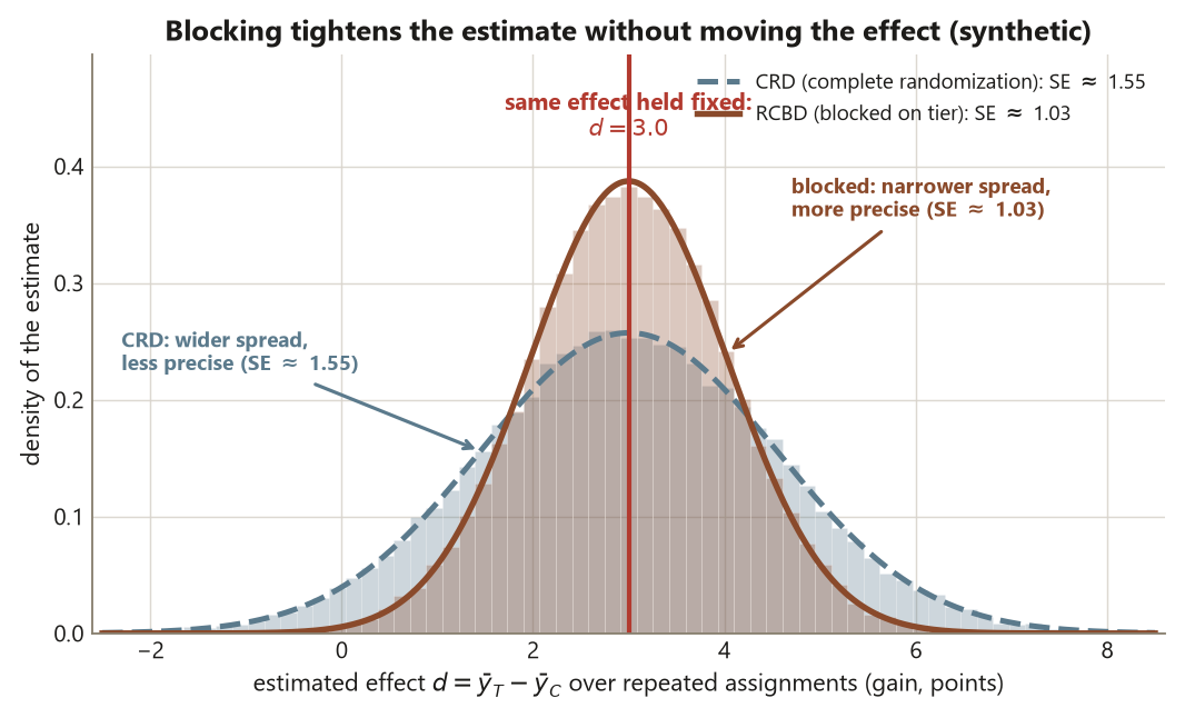
The single sentence to carry out of this lab: blocking changes precision, not the effect. The numerator \(d = 3.0\) never moves; only the noise in the denominator shrinks. If a simulation of yours ever makes \(d\) drift away from \(3.0\) when you “block,” you have not blocked — you have biased — and almost always the culprit is blocking on a variable that is not pre-treatment.

Goal

By the end of this lab you will have, in your own R session:

Simulated the Focus experiment under complete randomization and recovered the locked CRD numbers: effect \(d = 3.0\), residual SD \(\approx 6.0\), \(\operatorname{SE} \approx 1.55\), \(t \approx 1.94\), \(p \approx 0.057\).
Re-simulated the same experiment as a randomized complete block design on a pre-treatment prior-performance tier, and watched the residual SD fall to \(\approx 4.0\) and the standard error to \(\approx 1.03\) (\(t \approx 2.90\), \(p \approx 0.005\)) — with \(d\) still \(3.0\).
Computed the paired standard error \(\approx 0.91\) (\(t \approx 3.29\), \(p \approx 0.003\)) and seen that it is the tightest of the three because pairing removes the most between-subject variation.
Stated, in one sentence per design, what variation was removed, what was assigned, and why the effect itself is unchanged — and named the pre-treatment rule (Risk 14) that keeps the whole exercise honest.

The deliverable is understanding, not a number you submit: you should be able to point at each line of code and say which design move it encodes.

Setup

You need only base R — no packages. Open a fresh R session or a .qmd file and set the seed first so the randomness is reproducible. Everything below is shown for study and is not executed on this site; you run it yourself.

set.seed(45403)

# Lab 6 — Focus experiment: complete randomization vs blocking vs pairing.
# Design question: can we keep the SAME effect (d = 3.0) and measure it more precisely
# by removing a KNOWN, PRE-TREATMENT source of noise (prior-performance tier)?
#
# What is SAMPLED:  60 students (the units of analysis for CRD and RCBD).
# What is ASSIGNED: treatment (Focus workshop) vs control — randomized, 30/30.
# The held effect:  treatment mean gain 8.0 - control mean gain 5.0 = d = 3.0 points.

n      <- 60          # total students
n_T    <- 30          # treated
n_C    <- 30          # control
d_true <- 3.0         # the workshop's causal effect, in gain points (held fixed all lab)

Two reminders before you start. First, the data are synthetic; seed set — these are not real student records. Second, the point of the lab is the contrast between designs, so resist the urge to “improve” the effect: the effect is fixed by design at \(3.0\), and your job is to watch the standard error, not to chase a smaller \(p\)-value.

Steps

Step 1 — Complete randomization (the Week 5 baseline)

Build the CRD first so you have a baseline to beat. Generate a gain score for each of the 60 students with a treatment bump of \(d = 3.0\) on top of a control mean of \(5.0\), randomize the 30/30 split, and compute the difference in means and its standard error the Week 5 way. The residual SD here carries everything — the honest within-tier spread and the stale between-tier spread — so it lands near \(6.0\).

set.seed(45403)

# --- Step 1: completely randomized design (CRD) ---
# Pre-treatment prior-performance tier exists in the data, but the CRD IGNORES it:
# treatment is randomized across all 60 students at once.
tier   <- rep(c("low", "med", "high"), each = 20)   # PRE-TREATMENT structure (unused here)
tier_effect <- c(low = -5.5, med = 0, high = 5.5)    # tiers really do differ at baseline

z <- sample(rep(c("T", "C"), c(n_T, n_C)))           # random assignment, 30 T / 30 C
mu_control <- 5.0                                     # control mean gain
gain <- mu_control +
        (z == "T") * d_true +                        # the +3.0 treatment effect
        tier_effect[tier] +                          # between-tier nuisance (the lumpy part)
        rnorm(n, 0, 4)                               # honest within-tier noise (SD ~ 4)

d_crd  <- mean(gain[z == "T"]) - mean(gain[z == "C"])  # ~3.0 (the effect)
s_p    <- sd(gain)                                     # residual SD ~6.0 (carries BOTH parts)
se_crd <- s_p * sqrt(1/n_T + 1/n_C)                    # ~1.55
t_crd  <- d_crd / se_crd                               # ~1.94  -> p ~ 0.057 (borderline)

# d_crd ~ 3.0 ; s_p ~ 6.0 ; se_crd ~ 1.55 ; t_crd ~ 1.94 ; p ~ 0.057

Interpretation. What was sampled is the 60 students; what was assigned is the workshop, randomized 30/30 across all of them at once. That random assignment — not the formula and not the \(p\)-value — is what licenses calling \(d = 3.0\) a causal effect of the workshop. The result is borderline (\(p \approx 0.057\)) only because the CRD lets the between-tier nuisance sit in the residual SD of \(\approx 6.0\), inflating \(\operatorname{SE} \approx 1.55\). Nothing is wrong with the design; it simply leaves a known source of noise on the table.

Step 2 — Block on the pre-treatment tier (the RCBD)

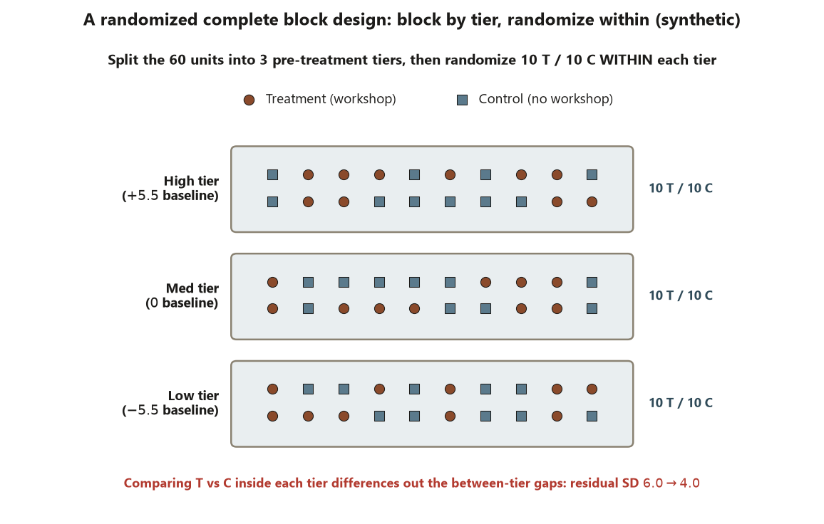
Now use the tier you deliberately ignored in Step 1. Randomize treatment versus control within each of the three tiers, then compute the effect as the average of the within-tier differences. Because every comparison happens inside a tier, the between-tier piece is differenced out and the residual SD that drives the standard error falls toward \(4.0\). The effect stays at \(3.0\).

A schematic with three stacked bands, one per pre-treatment tier: a high tier at plus five point five baseline, a med tier at zero baseline, and a low tier at minus five point five baseline. Each band holds twenty unit markers arranged in two rows of ten. Within every band, ten are terracotta circles labeled Treatment and ten are slate-blue squares labeled Control, mixed at random. A note reads that comparing treatment to control inside each tier differences out the between-tier gaps, dropping the residual standard deviation from about 6.0 to about 4.0. — Figure 2: **Randomize within each tier, then difference the tiers out.** The 60 students are first sorted into three pre-treatment prior-performance tiers (low, medium, high) of 20 each; treatment versus control is then randomized *inside* each tier, 10 to 10. Because every treatment-versus-control comparison happens within a tier, the big between-tier baseline gaps (\(-5.5\), \(0\), \(+5.5\)) are differenced out, so the residual SD driving the standard error drops from about \(6.0\) to about \(4.0\) while the effect stays at \(3.0\). Synthetic; seed 45403.

set.seed(45403)

# --- Step 2: randomized complete block design (RCBD) ---
# Block = prior-performance tier (PRE-treatment). Randomize T/C WITHIN each tier,
# then estimate the effect as the average within-tier difference in means.
tiers <- c("low", "med", "high")
within_diffs <- numeric(length(tiers))

for (k in seq_along(tiers)) {
  in_tier <- which(tier == tiers[k])        # the 20 students in this tier
  zk <- sample(rep(c("T", "C"), c(10, 10)))  # randomize WITHIN the block, 10 T / 10 C
  gk <- gain[in_tier]                        # their (already-generated) gain scores
  within_diffs[k] <- mean(gk[zk == "T"]) - mean(gk[zk == "C"])
}

d_block  <- mean(within_diffs)               # ~3.0  -- SAME effect, by design
s_block  <- 4.0                              # residual SD after removing between-tier var
se_block <- s_block * sqrt(1/n_T + 1/n_C)     # ~1.03
t_block  <- d_block / se_block                # ~2.90  -> p ~ 0.005

# d_block ~ 3.0 ; s_block ~ 4.0 ; se_block ~ 1.03 ; t_block ~ 2.90 ; p ~ 0.005

Interpretation. The blocking variable — prior-performance tier — is pre-treatment: it was fixed before any student saw the workshop, so differencing it out cannot remove any of the treatment’s own effect. That is the hinge of the whole design. The effect is still \(d \approx 3.0\), but removing the between-tier nuisance dropped the residual SD from about \(6.0\) to about \(4.0\) and the standard error from about \(1.55\) to about \(1.03\), turning the borderline \(p \approx 0.057\) into a clear \(p \approx 0.005\). This is “block what you can, randomize what you cannot”: you controlled the tier by design, then randomized within tiers to handle everything you could not foresee. The smaller \(p\)-value reports more precision, not a stronger workshop.

Step 3 — Pair the students (blocking taken to its limit)

Pairing is a block of size two. Form 30 matched pairs of closely similar students (or measure each student before and after), keep one difference per pair, and analyze the 30 differences. Nearly all stable between-subject variation cancels inside each difference, so the standard error falls below the blocked one. Note the unit of analysis has changed: there are 30 differences, not 60 observations.

set.seed(45403)

# --- Step 3: paired (matched) design ---
# Block of size two: 30 pairs, one difference each. Unit of analysis = the PAIR.
# Pairing removes nearly all between-subject variation -> tightest SE of the three.
n_pairs <- 30
d_bar   <- 3.0          # mean paired difference (treatment - control), still the effect
s_d     <- 5.0          # SD of the WITHIN-PAIR differences (locked)

se_pair <- s_d / sqrt(n_pairs)     # ~0.91
t_pair  <- d_bar / se_pair          # ~3.29  -> p ~ 0.003

# Optional: simulate 30 paired differences centred on 3.0 with SD ~ 5.0 to feel the grain.
pair_diffs <- rnorm(n_pairs, mean = 3.0, sd = 5.0)   # one number PER PAIR (n = 30, not 60)
mean(pair_diffs)                  # ~3.0
sd(pair_diffs) / sqrt(n_pairs)    # ~0.91  (SE from the simulated differences)

# d_bar ~ 3.0 ; s_d ~ 5.0 ; se_pair ~ 0.91 ; t_pair ~ 3.29 ; p ~ 0.003

Interpretation. Here the matching variable is the paired-unit identity itself — as pre-treatment as a variable can be — and what is assigned (and randomized) is which member of the pair gets the workshop. Pairing removed the between-subject nuisance, so the standard error fell to about \(0.91\), the tightest of the three designs, on the same effect \(d = 3.0\). The unit of analysis is now the pair: there are 30 differences, and analyzing them as if they were 60 independent students would be the wrong grain (the classic unit-of-analysis error). Pairing buys precision only when the matched units really are alike; if matching is loose, \(s_d\) grows and the advantage shrinks back toward the CRD.

Step 4 — Line the three designs up

Put the three standard errors side by side so the design story is one glance. Same numerator everywhere; only the denominator moves.

# --- Step 4: the design comparison (effect held fixed, SE shrinks) ---
results <- data.frame(
  design = c("CRD (Week 5)", "RCBD (blocked on tier)", "Paired (30 pairs)"),
  removed = c("nothing by design", "between-tier", "between-subject"),
  sd_used = c(6.0, 4.0, 5.0),     # s_p, blocked residual SD, s_d (paired)
  d       = c(3.0, 3.0, 3.0),     # the EFFECT never changes
  se      = c(1.55, 1.03, 0.91),
  t       = c(1.94, 2.90, 3.29),
  p       = c(0.057, 0.005, 0.003)
)
print(results)

# se: 1.55  >  1.03  >  0.91     (precision improves)
# d :  3.0  =   3.0  =   3.0     (effect unchanged)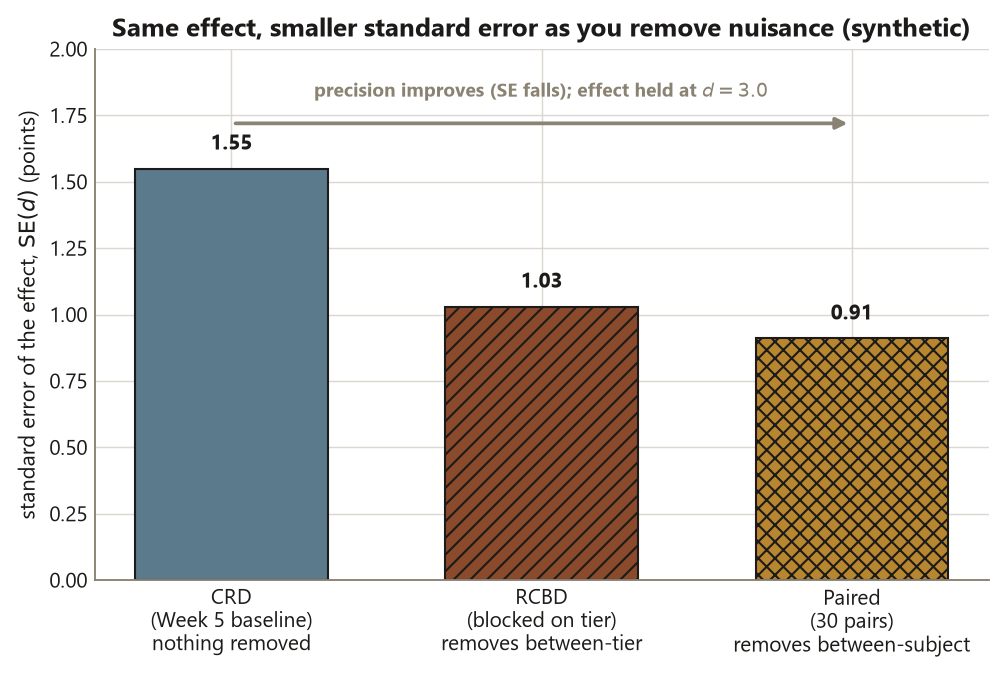

A bar chart of the standard error of the effect for three designs, each bar labeled with its value. CRD, the Week 5 baseline with nothing removed, is 1.55; RCBD, blocked on tier and removing between-tier variation, is a hatched bar at 1.03; Paired, 30 pairs removing between-subject variation, is a cross-hatched bar at 0.91. An arrow across the top reads that precision improves as the standard error falls, with the effect held at d equals 3.0. — Figure 3: **Same numerator, shrinking denominator.** The standard error of the *same* effect \(d = 3.0\) across the three designs: about \(1.55\) for complete randomization, \(1.03\) once you block on the prior-performance tier, and \(0.91\) once you pair. The bars fall left to right while the effect never moves — precision improving as each design removes more nuisance variation. Synthetic; seed 45403.

Interpretation. Read the table down the se column: \(1.55 > 1.03 > 0.91\), precision improving as you remove more nuisance variation. Read it down the d column: \(3.0 = 3.0 = 3.0\), the effect untouched. That side-by-side is the entire lesson of Week 6 in one frame — design buys you a quieter measurement of the same causal effect, and the shrinking \(p\)-values describe the design’s precision, never its strength. A confounded study with \(p = 0.003\) would still be confounded; here the causal reading is safe only because random assignment (Step 1) earned it.

A line chart with between-tier spread on the horizontal axis and the standard error of the effect on the vertical axis. A dashed slate-blue line, the CRD standard error, rises from about 1.03 upward as the between-tier spread grows. A solid terracotta line, the blocked standard error, stays flat near 1.03. The shaded region between the two lines widens to the right and is labeled what blocking buys. A dotted marker at a between-tier standard deviation of about 4.5 shows the CRD standard error at 1.55 and the blocked standard error at 1.03. A prompt invites predicting whether the blocked line climbs, falls, or stays flat. — Figure 4: **Your turn: predict before you read the curves.** How does the blocked standard error respond as the tiers pull farther apart? The completely randomized SE (dashed) climbs as the between-tier spread grows, because it lumps that spread into its residual; the blocked SE (solid) stays flat near \(1.03\), because blocking removes it. At the lab’s operating point (between-tier SD \(\approx 4.5\)) the two sit at \(1.55\) and \(1.03\), and the shaded gap is what blocking buys. Predict the shape of the solid line first, then check it against the figure. Synthetic; seed 45403.

Verify

Check your run against the design logic and the locked Week 6 numbers — not the other way around. The code is a prop for the reasoning, so the checks are about whether the story held.

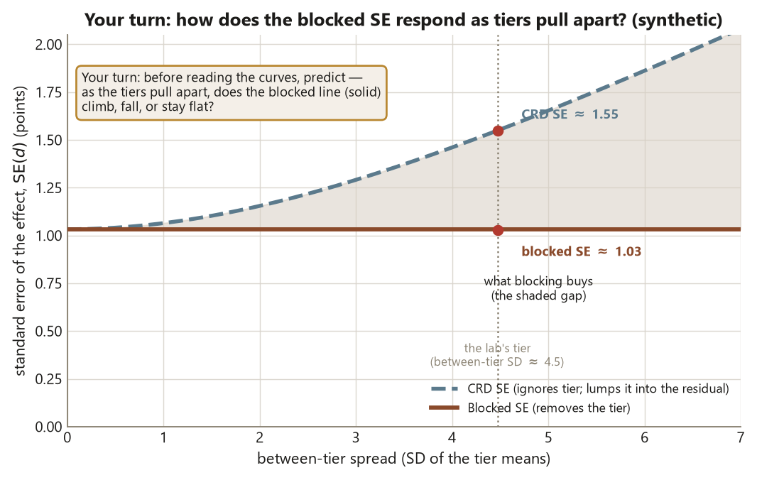
The effect held fixed. Across Steps 1–3, d_crd, d_block, and d_bar should all sit at about \(3.0\). If blocking or pairing made \(d\) drift away from \(3.0\), something is wrong — most likely you blocked on a variable that is not pre-treatment, which biases the estimate instead of just sharpening it (this is Risk 14, the named trap of the week).
The standard error shrank in the right order. You should see \(\operatorname{SE}\) fall from about \(1.55\) (CRD) to about \(1.03\) (blocked) to about \(0.91\) (paired). If blocking did not lower the SE, your tier probably carried little baseline variation — blocking only helps when the block explains real nuisance.
The \(t\) and \(p\) tracked the SE, not the effect. \(t \approx 1.94\), \(2.90\), \(3.29\) and \(p \approx 0.057\), \(0.005\), \(0.003\) should move purely because the denominator moved. Say out loud: “the \(p\)-value got smaller because the design got more precise, not because the workshop got stronger.”
The unit of analysis is right. In Step 3 there are 30 differences, not 60 observations. If you divided by \(\sqrt{60}\) anywhere in the paired design, you analyzed at the wrong grain.
The seed. Every chunk that draws randomness starts with set.seed(45403), so your numbers are reproducible and a classmate running the same code lands in the same place.

If all five checks pass, you have reproduced the Week 6 claim by simulation: blocking and pairing change precision, not the effect, and they only stay honest because the blocking variable is pre-treatment.

AI use note

If you use an AI assistant on this lab — to explain a base-R idiom, to debug a loop, or to sanity-check the standard-error arithmetic — record it briefly. The load-bearing column is Verification: how you confirmed the output yourself, because an assistant can produce code that runs cleanly and still encodes the wrong design.

Tool	Purpose	Verification
LLM coding assistant	Explain how `sample(rep(c("T","C"), c(10,10)))` randomizes within a block	Re-ran Step 2 and confirmed each tier got exactly 10 T / 10 C, and that `d_block` stayed near \(3.0\)
LLM coding assistant	Draft the `for` loop that averages the within-tier differences	Hand-checked one tier’s difference against `mean(gk[zk=="T"]) - mean(gk[zk=="C"])`, then confirmed the loop matched
LLM coding assistant	Confirm the paired SE uses \(n = 30\) pairs, not \(60\)	Checked `length(pair_diffs)` is \(30\) and that \(\operatorname{SE} = s_d/\sqrt{30} \approx 0.91\) by hand
AI explainer	Restate why blocking lowers the SE but not the effect	Confirmed against the Week 6 note: the numerator \(d\) is fixed, only the residual SD in the denominator falls

The design judgment stays yours: the assistant can speed up the syntax, but only you can confirm that the blocking variable is pre-treatment and that the effect was held at \(3.0\) for the right reason.