Week 15 — Final review & synthesis

The whole MAC Study thread, one picture

A scheduling note before anything else: this is the last class meeting of the term — Monday, December 7. There is a consultation day on Dec 8, and the cumulative final falls in the Dec 9–15 window (exact block TBA via Blackboard). Nothing on this page is graded, and nothing here previews content beyond what has already appeared in Weeks 1–13; any review guide Blackboard posts for the final is the authoritative one (see Public vs. graded below).

The week question

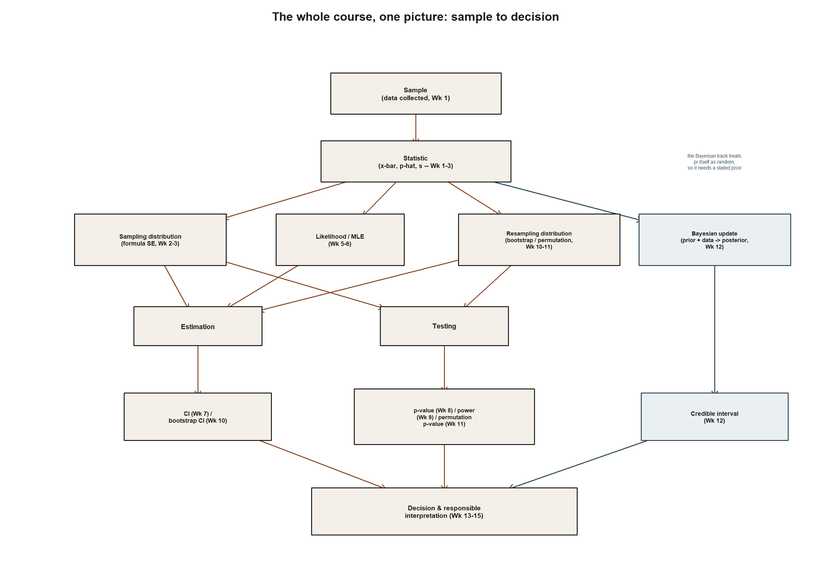
You have now built an entire toolkit — sampling distributions, estimators, standard errors, bias and variance, likelihood, maximum likelihood, confidence intervals, hypothesis tests, power, the bootstrap, randomization tests, and Bayesian updating — one week at a time, mostly on one running story, the MAC Study. This week asks a single question: what does it look like when you stop treating those as thirteen separate weeks and instead see them as one connected argument, with the same sample numbers passed from tool to tool? Today’s job is to walk that whole argument start to finish, once, out loud.

Why this matters

Every individual week necessarily narrowed its focus to make the new idea learnable on its own. That is the right way to build a toolkit, but it can leave the connections between tools implicit. In practice, nobody uses “just” a confidence interval or “just” a p-value; a real analysis moves fluidly between estimating, testing, quantifying uncertainty by simulation, and updating a prior belief — often on the same data set, asking different questions of it. Walking back through the MAC Study end to end shows that fluidity directly: the same n = 36 visit-duration sample and the same n = 100 usage-rate survey did real work in essentially every week from Week 2 onward. That is what makes this a course in statistical inference, not thirteen unrelated recipes.

Learning goals

By the end of this week you should be able to:

Retell the MAC Study’s inferential arc, Week 1 through Week 13, as one continuous story — explaining what each stage let you answer that the previous stage could not.
Trace how the same locked sample facts (x̄ = 49.8, s = 15.2, n = 36; p̂ = 0.38, n = 100) were reused, without being re-collected, across estimation, interval-building, testing, power, resampling, and Bayesian updating.
Distinguish, once more, the hypothetical “true” teaching-device world (Weeks 2, 4, 9) from the sample data actually in hand (everywhere else), and explain why conflating the two would undermine every inference made.
Compare the four inferential traditions previewed in Week 1 and reunited in Week 13 on the shared question of the MAC usage rate π.
Identify which weeks build vocabulary (1, 3), which build machinery (2, 4–6, 9), and which apply that machinery directly (7, 8, 10–13) — that structure matters more than any single formula.

Core vocabulary

This week deliberately introduces no new terms. Instead, here are the words that quietly carried the whole course:

Parameter vs. statistic. μ and π are fixed, unknown facts about a population (Week 1); x̄, s, and p̂ are numbers computed from a sample, and vary from sample to sample (Weeks 1–3).
Standard error. How much a statistic bounces around across hypothetical repeated samples (Week 3) — the ingredient every CI, test statistic, and power calculation in Weeks 7–9 is built from.
Likelihood. A function of the parameter, for fixed observed data (Weeks 5–6) — never a probability distribution over the parameter, a distinction kept until Week 12 deliberately introduces a prior.
Confidence, significance, and power. Three faces of the same standardized-distance idea, aimed at a range, a decision, and a detection rate (Weeks 7–9).
Resampling and permutation. Using the computer to approximate a sampling distribution directly from the data in hand (bootstrap, Week 10) or reshuffling group labels for a null distribution (permutation, Week 11).
Prior, likelihood, posterior. The Bayesian update (Week 12): a prior belief about π, updated by data into a posterior that is a full distribution over π, not a single point estimate.

Concept development

Thirteen weeks of tools collapse into one connected shape once you see them side by side. Keep this picture in mind as the anchor for the four “acts” below.

A large flow diagram. Sample flows down to Statistic. Statistic branches into three boxes: sampling distribution formula S E weeks 2 to 3, likelihood or M L E weeks 5 to 6, and resampling distribution bootstrap or permutation weeks 10 to 11; it also branches to a separate Bayesian update box, week 12, colored distinctly to mark it as a separate track. Sampling distribution and resampling distribution both feed into two boxes, Estimation and Testing; likelihood or M L E feeds into Estimation only. Estimation flows to a CI or bootstrap CI box; Testing flows to a p-value, power, or permutation p-value box; the Bayesian update box flows to a Credible interval box. All three of those boxes converge into a final box, Decision and responsible interpretation, weeks 13 to 15. — Figure 1: **The whole course, one picture: sample to decision.** Every sample becomes a statistic, whose sampling behavior is captured by a formula, a likelihood argument, or a resampling scheme, or — on a separate Bayesian track — combined with a stated prior; each route feeds into estimation or testing, produces an interval, a p-value, a power figure, or a credible interval, and lands in the same decision-and-interpretation step.

What the figure shows (non-visual equivalent). Every sample produces a statistic; that statistic’s behavior across hypothetical repeated samples is described by a formula-based sampling distribution (Weeks 2–3), by a likelihood/MLE argument (Weeks 5–6), or by directly resampling or permuting the data (Weeks 10–11). A separate Bayesian track (Week 12) instead treats the parameter itself as random, combining a stated prior with the same data. The first three routes feed into either estimation (producing a CI, Week 7, or a bootstrap CI, Week 10) or testing (producing a p-value, Week 8, a power figure, Week 9, or a permutation p-value, Week 11); the Bayesian route produces a credible interval (Week 12) directly. All routes converge on the same final step: a decision and a responsible, assumption-aware interpretation (Weeks 13–15).

Act one: setting up the question (Weeks 1–4)

The term opened with a distinction everything else depends on: a population has fixed, unknown parameters (μ, mean MAC visit duration; π, the weekly usage rate), and a sample is what you actually observe (Week 1). Week 2 made that concrete by simulating — under a hypothetical stipulated truth, Normal(μ = 48, σ = 15) — what a sampling distribution of x̄ looks like across many samples of n = 36; that simulation is a teaching device only, never confused with the real, unknown μ the course learns about honestly elsewhere. Week 3 named the spread: SE(x̄) = σ/√n = 15/6 = 2.5, and SE(p̂) = √(p̂(1−p̂)/n) ≈ 0.0485. Week 4 asked whether an estimator is systematically off-target (bias) and how much it bounces around its own average (variance): the (n−1) divisor corrects exactly the bias (−6.25) the plain (1/n) divisor introduces, and the shrinkage example showed a lower-variance estimator (Var = 5.0625) can still be worse overall (MSE = 28.1025) than the unbiased x̄’s MSE of 6.25.

Act two: two routes to an estimate, then quantifying it (Weeks 5–9)

Weeks 5–6 added a second lens: instead of “what estimator has good long-run properties,” likelihood asks “which parameter value makes the observed data most plausible.” Week 5’s small pilot (n = 5, k = 2) compared the kernel π²(1−π)³ by hand at π = 0.2, 0.4, 0.6 (0.02048, 0.03456, 0.02304 — π = 0.4 highest), foreshadowing Week 6’s Binomial MLE π̂ = 2/5 = 0.4 and Normal MLE μ̂ = x̄ = 50 (from visits 52, 46, 58, 41, 53) — both agreeing with the intuitive “just average” answer.

A point estimate still hides its uncertainty, which Weeks 7–9 addressed with Week 3’s standard errors. Week 7 turned estimate plus SE into a range: 95% CI for μ, 49.8 ± 1.96(2.5) = (44.9, 54.7); for π, 0.38 ± 1.96(0.0485) = (0.285, 0.475). Week 8 turned the same ingredients toward a yes/no question — is last year’s baseline of 45 minutes still consistent? — z = (49.8 − 45)/2.5 = 1.92, two-sided p ≈ 0.0548, borderline, failing to reject at α = 0.05. Week 9 asked what a test alone cannot: if μ really were 50, how likely is detection? Critical value 45 + 1.645(2.5) = 49.11; power = P(Z > −0.355) ≈ 0.639 (β ≈ 0.361). Confidence, significance, and power are three questions asked of the same standardized distance, aimed at a range, a decision, a detection rate.

Act three: letting the computer do the sampling (Weeks 10–11)

Weeks 10–11 asked what happens when the computer approximates sampling behavior directly from data. Week 10’s bootstrap resampled the n = 36 sample using the sample SD s = 15.2, producing a percentile 95% CI ≈ (44.84, 54.76) — close to but not identical to Week 7’s (44.9, 54.7), reflecting bootstrap SE ≈ 2.53 versus known-σ SE = 2.5. Week 11’s workshop-vs-control comparison (n₁ = n₂ = 20, difference 7.3 minutes) built a null distribution by permuting group labels; the permutation p-value closely matched the normal-approximation cross-check (z ≈ 2.31, p ≈ 0.021), as expected when group sizes and spreads are close.

Act four: a different object of inference (Week 12), then the reunion (Week 13)

Week 12 changed the question most fundamentally: Bayesian inference treats π itself as having a distribution that data updates. Starting from Beta(a = 3, b = 7) (prior mean 0.30) and the full survey (n = 100, k = 38), Bayes’ rule gives posterior Beta(41, 69), mean 41/110 ≈ 0.373, 95% credible interval ≈ (0.283, 0.463) — the same data drove both this posterior and the Week 3/7 frequentist p̂ = 0.38; only the question asked of it changed.

Week 13 reunited all four traditions on π: frequentist p̂ = 0.38, CI (0.285, 0.475); likelihood/MLE π̂ = 0.4 from the separate small pilot; simulation-based logic cross-checking intervals and p-values computationally; and Bayesian posterior mean ≈ 0.373, credible interval (0.283, 0.463) — closer to the frequentist estimate than the prior’s 0.30, since n = 100 outweighed a gentle prior. None is “the” correct answer; each turns the same evidence into a different, defensible kind of statement about π.

Putting it together

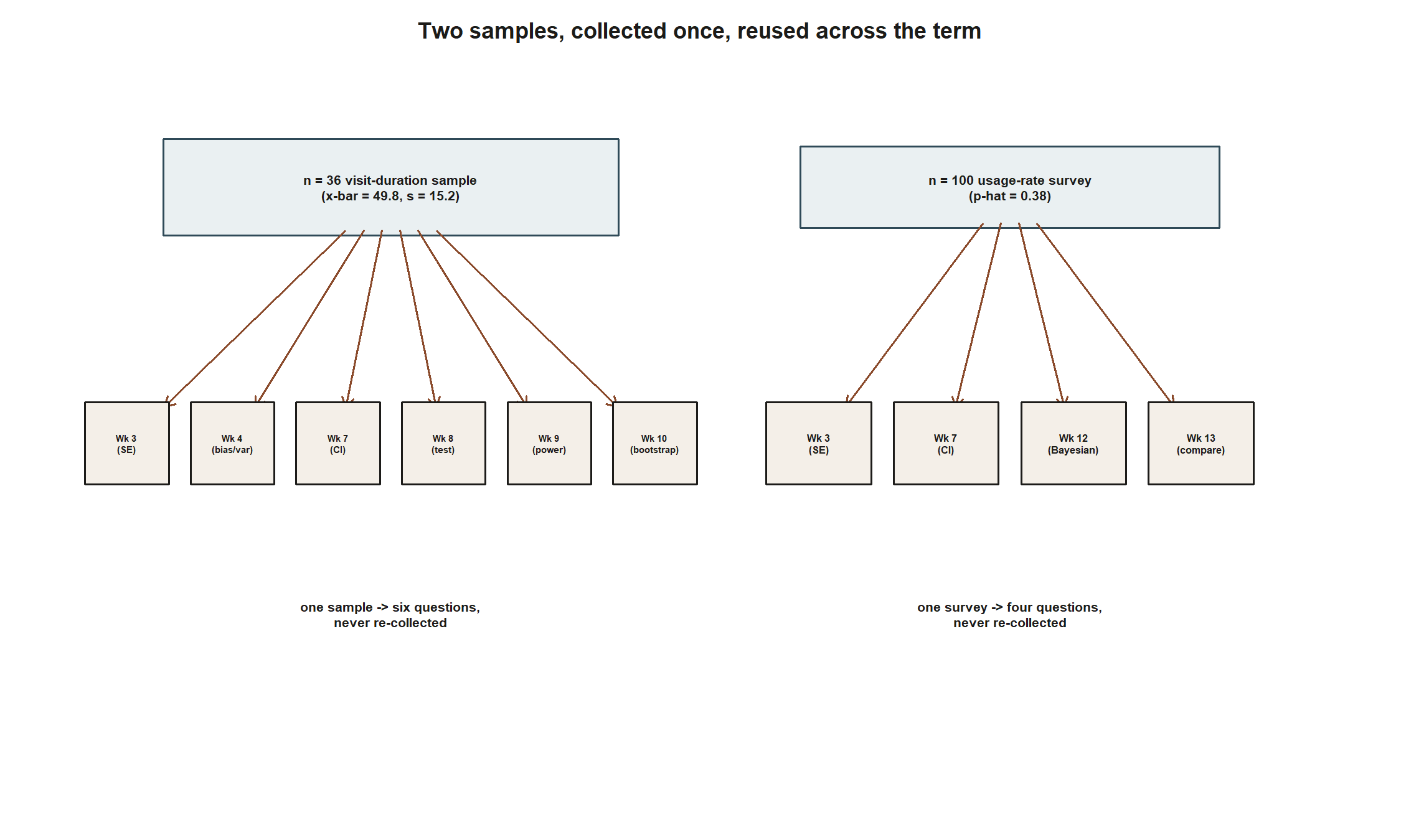
Look at how few numbers did all this work. The n = 36 visit-duration sample alone supported Weeks 3, 4, 7, 8, 9, and 10 — six questions, one sample, never re-collected. The n = 100 usage-rate survey supported Weeks 3, 7, 12, and 13. The small illustrative pilots (n = 5 for the proportion, five visits for the mean) existed for one purpose each — making Weeks 5–6’s by-hand arithmetic tractable — and were narrated as separate from, and prior to, the full samples used elsewhere. Holding that separation is the single habit this course has asked you to build.

Two fan-out diagrams side by side. On the left, a box labeled n equals 36 visit-duration sample, x-bar equals 49.8, s equals 15.2, with arrows fanning down to six small boxes labeled week 3 SE, week 4 bias slash variance, week 7 CI, week 8 test, week 9 power, and week 10 bootstrap. On the right, a box labeled n equals 100 usage-rate survey, p-hat equals 0.38, with arrows fanning down to four small boxes labeled week 3 SE, week 7 CI, week 12 Bayesian, and week 13 compare. — Figure 2: **Two samples, collected once, reused across the term (synthetic).** The n = 36 visit-duration sample (x̄ = 49.8, s = 15.2) alone did the work behind Weeks 3, 4, 7, 8, 9, and 10; the n = 100 usage-rate survey (p̂ = 0.38) alone did the work behind Weeks 3, 7, 12, and 13 — six and four separate questions asked of two samples that were each collected exactly once.

Worked examples

Worked example — MAC Study: the same π, four ways, one table

Setup. Let π denote the unknown population usage rate. Four traditions each produce a summary of π from the same evidence base (full survey n = 100, k = 38; likelihood/MLE row uses the separate small pilot n = 5, k = 2):

Before the four-row table, see the frequentist and Bayesian rows as two paths starting from the same data:

Two side-by-side vertical flow diagrams. The left panel, titled frequentist path weeks 3 and 7, flows: sample n equals 100, k equals 38; down to p-hat equals 0.38; down to 95 percent CI 0.285 to 0.475; down to a box reading long-run capture-rate claim about the procedure, not a probability about pi. The right panel, titled Bayesian path week 12, flows: sample n equals 100, k equals 38, plus prior Beta 3 comma 7; down to posterior Beta 41 comma 69; down to 95 percent credible interval 0.283 to 0.463; down to a box reading direct probability statement about pi itself, given prior and data. — Figure 3: **Two paths, the same data, different questions (synthetic).** The frequentist path turns the n = 100, k = 38 survey into p̂ = 0.38 and a 95% CI (0.285, 0.475), a claim about the procedure’s long-run behavior; the Bayesian path combines the same survey with a Beta(3, 7) prior into a posterior Beta(41, 69) and a 95% credible interval (0.283, 0.463), a direct probability statement about π itself.

What the figure shows (non-visual equivalent). Both paths start from the identical survey (n = 100, k = 38). The frequentist path stops at p̂ = 0.38 and a 95% CI of (0.285, 0.475), a statement about how often the procedure would capture π across repeated sampling — never a probability about this one interval. The Bayesian path adds a stated prior, Beta(3, 7), updates it with the same data to a posterior Beta(41, 69), and reports a 95% credible interval (0.283, 0.463), which — because π now has a full distribution — licenses a direct probability statement about π itself. The two intervals land close together because the prior is comparatively weak relative to n = 100.

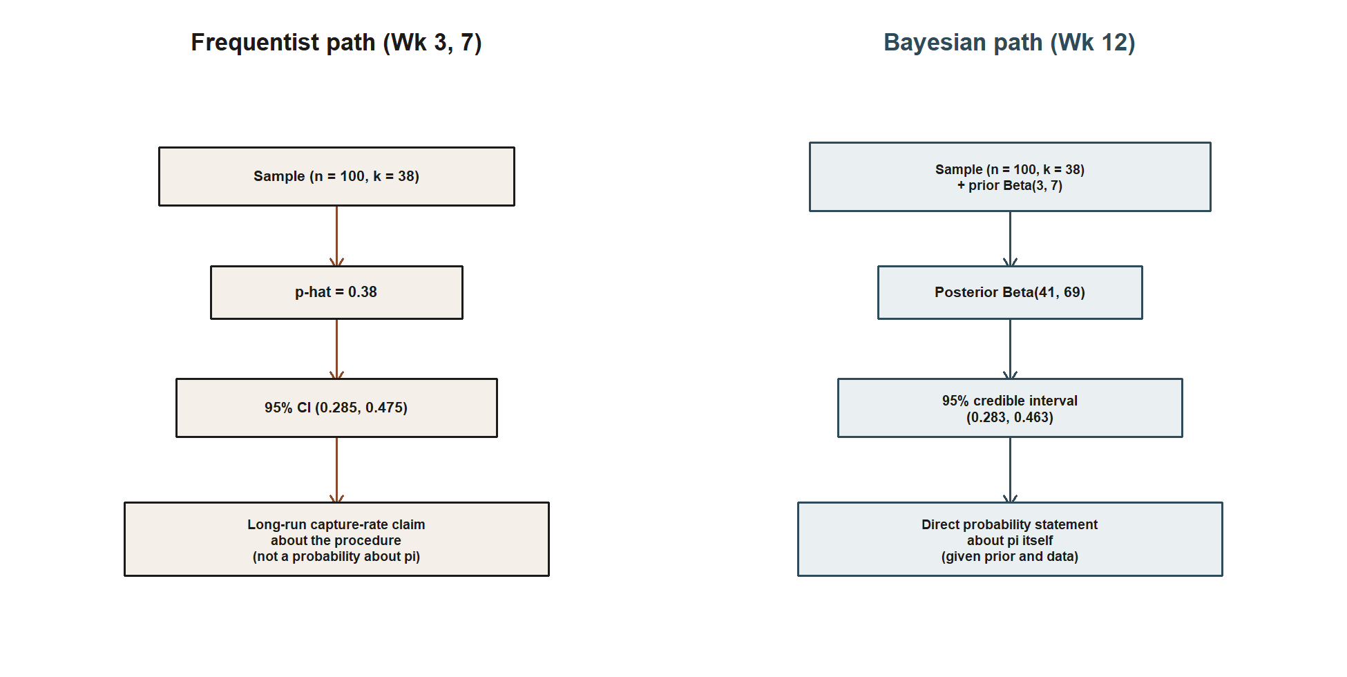
The table below fills in all four traditions numerically, including the likelihood/MLE and simulation-based rows the two-panel figure above does not cover.

Framework	Point summary	Interval	What it treats as random
Frequentist (Weeks 3, 7, 8)	p̂ = 0.38	95% CI (0.285, 0.475)	the estimate, across hypothetical repeated samples
Likelihood / MLE (Weeks 5–6)	π̂ = k/n = 0.4 (pilot n = 5)	— (not built this term)	none — a plausibility ranking over π, for fixed data
Simulation-based (Weeks 10–11)	resampled/permuted estimate ≈ matches formula-based results	bootstrap-style interval, same shape as frequentist CI	the resampling/reshuffling process itself
Bayesian (Week 12)	posterior mean ≈ 0.373	95% credible interval (0.283, 0.463)	π itself, via a full posterior distribution

Numeric check. The frequentist CI, 0.38 ± 1.96(0.0485) = (0.285, 0.475), and the Bayesian credible interval, 0.373 ± 1.96(0.0459) = (0.283, 0.463), overlap heavily and are similar in width (both about 0.18–0.19), even though they mean different things — a long-run capture-rate claim about the procedure, versus a direct probability statement about where π lies, now licensed because π has a distribution. The posterior mean 0.373 sits slightly below the raw p̂ = 0.38 because the prior’s mean (0.30) pulls that way.

Interpretation. No row in this table is wrong. Each answers a genuinely different question about the same π — a long-run procedure property, a plausibility ranking, a resampling-based approximation, or an updated belief — and choosing among them is about which question you need answered, not which one is “true.”

Worked example — transfer: reviewing a different recurring data set end to end (synthetic; seed set)

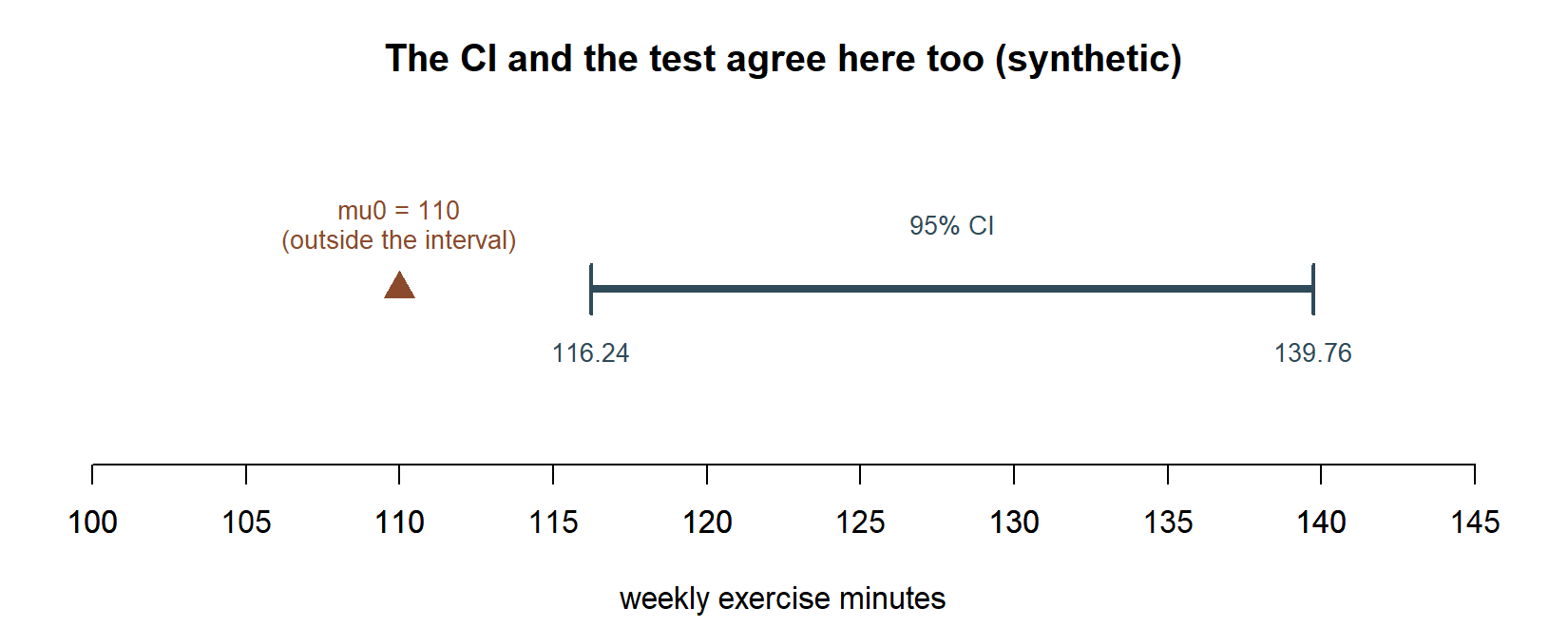
Synthetic; seed set. A separate campus wellness study samples n = 25 students on weekly exercise minutes, x̄ = 128, and (known-σ simplification) σ ≈ 30, so SE(x̄) = 30/√25 = 6. The 95% CI (Week 7’s recipe):

\[ 128 \;\pm\; 1.96(6) \;=\; 128 \;\pm\; 11.76 \;=\; (116.24,\; 139.76). \]

A test (Week 8’s recipe) of H0: μ = 110 against Ha: μ ≠ 110 gives z = (128 − 110)/6 = 3.00, two-sided p ≈ 2(1 − Φ(3.00)) ≈ 0.0027 — a clear rejection at α = 0.05, unlike the MAC Study’s borderline Week 8 case. Interpretation. The same recipes, in an unrelated synthetic context, produce a clean rejection instead of a near-miss — the machinery transfers perfectly; only the conclusion changes with how far the data sits from the reference value.

A number line from 100 to 145 weekly exercise minutes. A thick bracket runs from 116.24 to 139.76, labeled 95 percent CI. A triangular marker sits at 110, to the left of and outside the bracket, labeled mu-zero equals 110, outside the interval. — Figure 4: **The CI and the test agree here too (synthetic; seed set).** The transfer example’s 95% CI, (116.24, 139.76), sits entirely above μ0 = 110 — the null value falls outside the interval, matching the test’s rejection at α = 0.05 (z = 3.00, p ≈ 0.0027), the mirror image of the MAC Study’s borderline case (Week 8), where μ0 sat just inside the interval.

set.seed(35103)

# Visit-duration thread: recap the chain from one sample (Weeks 3, 7, 8, 9, 10)
xbar <- 49.8; s <- 15.2; n <- 36
se_known_sigma <- 15 / sqrt(n)
se_bootstrap   <- s / sqrt(n)
ci_wk07   <- xbar + c(-1, 1) * 1.96 * se_known_sigma
z_wk08    <- (xbar - 45) / se_known_sigma
crit_wk09 <- 45 + 1.645 * se_known_sigma
ci_wk07; z_wk08; crit_wk09; se_bootstrap

# Usage-rate thread: frequentist vs. Bayesian summary, side by side (Week 13)
phat <- 0.38; n_survey <- 100
se_phat <- sqrt(phat * (1 - phat) / n_survey)
ci_freq <- phat + c(-1, 1) * 1.96 * se_phat

a_prior <- 3; b_prior <- 7; k <- 38
a_post <- a_prior + k
b_post <- b_prior + (n_survey - k)
post_mean <- a_post / (a_post + b_post)
post_sd   <- sqrt((a_post * b_post) / ((a_post + b_post)^2 * (a_post + b_post + 1)))
ci_bayes  <- post_mean + c(-1, 1) * 1.96 * post_sd
ci_freq; post_mean; ci_bayes

A common mistake

Treating the term’s thirteen tools as a menu of unrelated recipes to memorize separately, rather than as one connected argument that reuses the same handful of ingredients. A student who can recite the CI formula and the p-value formula in isolation, but cannot say why both use the same standardized distance, or why the bootstrap CI came out close to but not identical to the Week 7 CI, has memorized formulas without absorbing the course’s point. A closely related version, worth naming one last time: conflating the hypothetical “true” values used only as teaching devices (μ = 48, σ = 15, π = 0.35 in Weeks 2, 4, 9) with the real sample data every actual inference was built from (x̄ = 49.8, s = 15.2, p̂ = 0.38). Every real analysis this course modeled worked strictly from sample data in hand, never from a peeked-at “true” answer — that is the entire premise of statistical inference rather than merely describing a fully known model.

Low-stakes self-checks (ungraded)

Without looking back, write out the visit-duration numbers from memory (n, x̄, s) and the usage-rate survey’s numbers (n, k, p̂), then check against Week 1’s and Week 3’s notes.
For each of Weeks 7 through 12, name in one sentence the question that week answers (not the formula) — for example, “Week 8 asks whether a specific hypothesized value is still consistent with the data.”
Explain why the Week 7 CI, (44.9, 54.7), and the Week 10 bootstrap CI, (44.84, 54.76), are close but not identical, using the distinction between a known σ and an estimated s.
Using the transfer example’s numbers (x̄ = 128, SE = 6), sketch what a Week-9-style power calculation against μ = 135 would need as ingredients, without computing it.
Pick any two of the four frameworks compared in Week 13 and state what each treats as random and what each treats as fixed — a clean way to keep the four traditions distinct for the final.

Reading and source pointer

For a compact end-of-term pass, MIT OCW 18.05’s treatment across sampling distributions, estimation, testing, and Bayesian inference is worth skimming as a whole rather than chapter by chapter, since this week’s value is in the connections between topics. As an optional lighter pass, useful for a gentler review of the most foundational ideas (population vs. sample, standard errors, confidence intervals) before the final, OpenIntro IMS’s introductory inference chapters cover much of the same ground at an easier pace. These notes are the course’s own synthesis, grounded in but not copied from the sources.

Public vs. graded

These notes, the examples, and the practice here are public and ungraded — study material only. No graded prompts, answer keys, rubrics, point values, or due dates appear on this site. Graded inference checkpoints, quizzes, homework, labs, the midterm, the project, and the final live in Blackboard (the LMS), which is authoritative for due dates, submissions, and grades. If this page and Blackboard ever disagree, follow Blackboard.

On the final specifically: the cumulative final falls in the Dec 9–15 window, exact block TBA via Blackboard. Coverage, format, and review materials are handled there, not here.

Looking ahead

There is no Week 16. This synthesis closes the note sequence; from here, Blackboard becomes the sole channel for consultation-day (Dec 8) logistics and the final-exam window (Dec 9–15). The inference project (Week 14) remains the term’s other synthesis point — applying at least two frameworks to a new question of the student’s own choosing — and this walk back through the MAC Study is meant to support exactly that transfer.