Week 1 — What statistical inference is
From a sample in hand to a responsible claim about a population
The week question
You already know how to compute a mean, a proportion, and a standard deviation from a batch of numbers. This week asks a different question: once you have those numbers, what are you allowed to say, and how confident are you allowed to be? Statistical inference is the disciplined practice of reasoning from a sample you actually observed to a claim about a population or process you did not fully observe — and of being honest, in a quantifiable way, about how uncertain that claim is.
Why this matters
Almost no question you actually care about can be answered by measuring everyone or everything. A campus center cannot track every visit by every student for all time; a pollster cannot ask every voter; a factory cannot destructively test every unit it ships. Someone collects a sample instead — necessarily partial, necessarily noisy — and then wants to say something responsible about the whole. That gap between “what the sample shows” and “what is true about the population” is exactly the gap this course is built to cross, carefully and with explicit uncertainty attached. Getting it wrong is the difference between a defensible claim and a false confidence that a sample happened to look a particular way just by chance.
This first week does not derive any formula. It builds the vocabulary every later week depends on. If the population-vs-sample and parameter-vs-statistic distinctions are solid now, confidence intervals (Week 7), hypothesis tests (Week 8), and Bayesian updating (Week 12) will read as variations on one theme rather than as unrelated recipes.
Learning goals
By the end of this week, you should be able to:
- State, in your own words, what “statistical inference” means and how it differs from simply describing a data set (descriptive statistics) or computing a probability from a fully specified model (probability).
- Distinguish a population from a sample, and a parameter from a statistic.
- Distinguish an estimator (a procedure/rule) from an estimate (the number that procedure produces on a particular sample).
- Explain, informally, why a sample statistic is expected to vary from sample to sample, even when the population does not change.
- Name the four inferential traditions this course studies side by side — frequentist, likelihood-based, simulation-based, and Bayesian — and describe, at a preview level only, what each one treats as the object of interest.
Core vocabulary
- Population. The complete collection of individuals, units, or outcomes you ultimately want to say something about — often too large, too costly, or logistically impossible to measure in full.
- Sample. A subset of the population that you actually observe and measure. Everything you compute in this course is computed from a sample.
- Parameter. A fixed (though typically unknown) numerical fact about the population — for example, a population mean \(\mu\) or a population proportion \(\pi\). A parameter does not have a sampling distribution; it is simply true, and simply unknown to the analyst.
- Statistic. A number computed from a sample — for example, a sample mean \(\bar{x}\) or a sample proportion \(\hat{p}\). Unlike a parameter, a statistic varies: a different sample would generally give a different statistic, even from the exact same population.
- Estimator. The general rule or procedure used to produce an estimate from data (for example, “take the arithmetic mean of the sample”) — a recipe that can, in principle, be applied to any sample of the appropriate kind.
- Estimate. The specific numerical output of an estimator applied to one particular, already-collected sample. “The sample mean” is an estimator; “\(\bar{x} = 49.8\)” is an estimate.
- Sampling variability. The fact that a statistic computed from one sample will generally differ from the same statistic computed from a different sample drawn from the same population — not a mistake, but an expected, quantifiable consequence of observing only part of a population.
- Inference. Using a statistic (and an explicit accounting of its sampling variability) to make a defensible, appropriately hedged statement about the population parameter that generated it.
Concept development
From describing data to inferring about a population
Descriptive statistics summarizes the data you have: a mean, a median, a histogram, a proportion. None of that requires any assumption about where the data came from. Statistical inference asks for something more ambitious: given this sample, what can we responsibly claim about the population it was drawn from? That extra step needs new machinery — a model for how sampling variability behaves, and a language for expressing uncertainty (confidence intervals, p-values, posterior distributions) rather than just a single summary number.
It helps to keep three activities distinct, because this course moves between all three:
- Probability starts from a fully specified model (for example, “assume a fair coin”) and asks what outcomes are likely. The population/model is known; you reason forward to what data might look like.
- Descriptive statistics starts from data you already have and summarizes it: no claim about a broader population is made.
- Statistical inference starts from data you already have and reasons backward to what the unknown population parameter probably is. The population/model is unknown; you reason backward from data to what generated it.
This course sits in the third activity, drawing on tools from the first two: a probability model tells you how a statistic should behave under stated assumptions, and that behavior is what licenses an inferential statement about the unknown parameter.
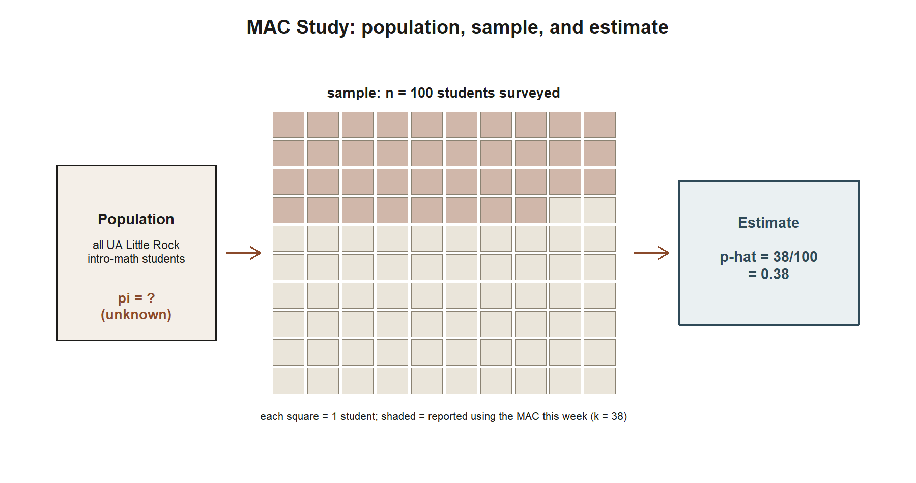
Setting up the MAC Study: an unknown population behind every sample
This course returns all term to a single running example, “the MAC Study” — a research team studying use of UA Little Rock’s Math Assistance Center (MAC). The MAC Study is entirely synthetic (invented for teaching), built to feel like a realistic small research project, and every number attached to it is fixed and reused deliberately across weeks so you can watch the same numbers support increasingly sophisticated methods.
The research team cares about two unknown population quantities:
- \(\mu\), the population mean number of minutes a student spends on a MAC visit in a given week.
- \(\pi\), the population proportion of students in a large intro math course who use the MAC at least once in a given week (a “usage rate”).
Both \(\mu\) and \(\pi\) are parameters: fixed facts about the full population of students and visits, and the research team does not know either one. Nobody can track every visit by every student, so the team cannot simply compute \(\mu\) and \(\pi\) directly — they can only sample.
To make certain teaching points concrete later in the course (simulating a sampling distribution in Week 2, computing statistical power under a stipulated alternative in Week 9, and illustrating estimator bias/variance in Week 4), this course sometimes stipulates a hypothetical “true” version of this world: visit duration hypothetically following a Normal(\(\mu = 48\), \(\sigma = 15\)) distribution, and weekly usage hypothetically following a Bernoulli(\(\pi = 0.35\)) distribution. Keep this hypothetical device separate from real inference: in an actual analysis, the whole point is that \(\mu\) and \(\pi\) are not known, and no analyst is allowed to peek at a “true” value. The hypothetical world is a teaching prop used only in the weeks named above, always flagged clearly when it appears.
What the research team actually has, in every estimation, testing, bootstrap, permutation, and Bayesian week from here on, is sample data: real (synthetic-but-fixed) numbers collected as an actual analyst would collect them, without knowing the true parameter values. This week, it is enough to know such samples exist and that the rest of the course is about extracting responsible, quantified claims from them — the specific sample numbers (like \(\bar{x} = 49.8\) and \(\hat{p} = 0.38\)) start doing real work beginning in Week 2 and become central from Week 7 onward.
Estimator vs. estimate, and why sampling variability is not an error
A frequent point of confusion for students new to inference is treating “the formula” and “the number it produced” as the same thing. They are not. “Compute the sample mean” is an estimator: a general instruction that could be applied to any sample of visit durations the research team might have collected. Once applied to one particular sample, it produces an estimate: one specific number.
This distinction matters because the estimator is what has statistical properties — it is the estimator (not any single estimate) that can be unbiased, have a certain standard error, or converge to the truth as \(n\) grows. A single estimate is just one number; it makes no sense to ask whether one number, by itself, is “biased.” Later weeks (especially Week 3 on standard errors and Week 4 on bias/variance/MSE) study these properties directly.
It also explains why two research teams, each properly sampling the same population, will almost never get identical statistics. If the MAC Study team resurveyed a fresh batch of 100 students next week, the new sample proportion would almost certainly not equal 0.38 again — not because anyone made a mistake, but because a sample proportion is itself a random quantity that varies from sample to sample. This sampling variability is not noise to be eliminated; it is a fact to be measured, and measuring it (via the standard error, starting in Week 3) is what allows an honest statement of uncertainty rather than a false claim of exactness.
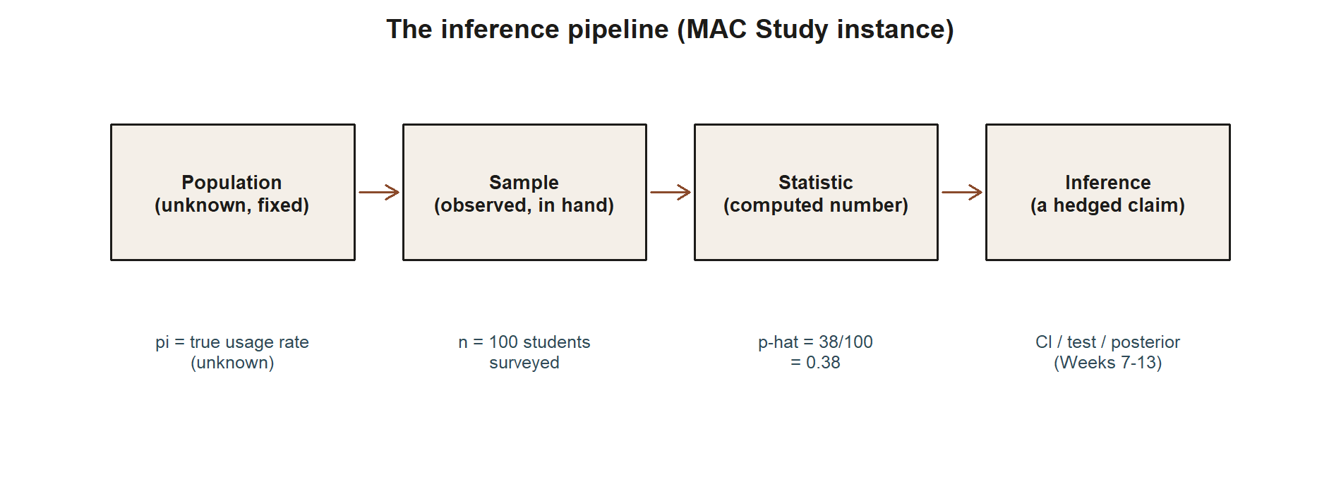
Seeing the whole pipeline at a glance
Table 1. The inference pipeline, MAC Study instance. Every question this course asks moves through the same four stages, left to right. Population and parameter are fixed but unknown; sample and statistic are what an actual research team can get their hands on.
POPULATION            SAMPLE                  STATISTIC              INFERENCE
(unknown, fixed)  →   (observed, in hand)  →  (computed number)  →  (a hedged claim)
The same pipeline, drawn as a figure, with this week’s MAC Study numbers attached to each stage:
| Stage | What it is | MAC Study instance |
|---|---|---|
| Population | Every student’s true MAC behavior — never fully observed | all UA Little Rock intro-math students |
| Parameter | A fixed, unknown numerical fact about the population | \(\pi\) = true weekly usage rate; \(\mu\) = true mean visit minutes |
| Sample | The subset actually surveyed or measured | \(n = 100\) students surveyed this week |
| Statistic | A number computed from the sample — itself random, since a different sample gives a different number | \(\hat{p} = k/n = 38/100 = 0.38\) |
| Inference | A quantified, hedged claim about the parameter, built from the statistic plus its sampling variability | a confidence interval, test, or posterior for \(\pi\) (Weeks 7–13) |
Read the diagram left to right and the table top to bottom together: the population and its parameter sit at the far left, permanently out of reach; everything this course teaches how to compute lives in the sample and statistic columns; and everything this course teaches how to say responsibly lives in the inference column on the right. Every method in every later week is a different way of building that last arrow — turning a statistic into a defensible statement about the parameter that produced it.
A preview of four ways to reason from sample to population
This course is intentionally pluralistic: rather than teaching a single inferential framework as the correct one, it studies four traditions side by side and asks what each one treats as its central object. This is only a preview — none of these is derived or used formally until its dedicated week.
- Frequentist inference (Weeks 2–3, 7–9, 11) treats the parameter as a fixed, unknown constant and studies the long-run behavior of a procedure across many hypothetical repetitions of sampling. A confidence interval is a property of the procedure used to build it, not a probability statement about one particular interval.
- Likelihood-based inference (Weeks 5–6) asks which parameter values make the data actually observed most plausible, treating the likelihood function as a function of the unknown parameter for fixed data.
- Simulation-based inference (Weeks 2, 10, 11) uses computation — resampling, permutation, and other forms of simulation — to approximate a statistic’s behavior directly from the data, rather than a closed-form formula.
- Bayesian inference (Week 12) treats the unknown parameter as having a probability distribution that is updated by data, moving from a prior belief to a posterior belief via Bayes’ rule.
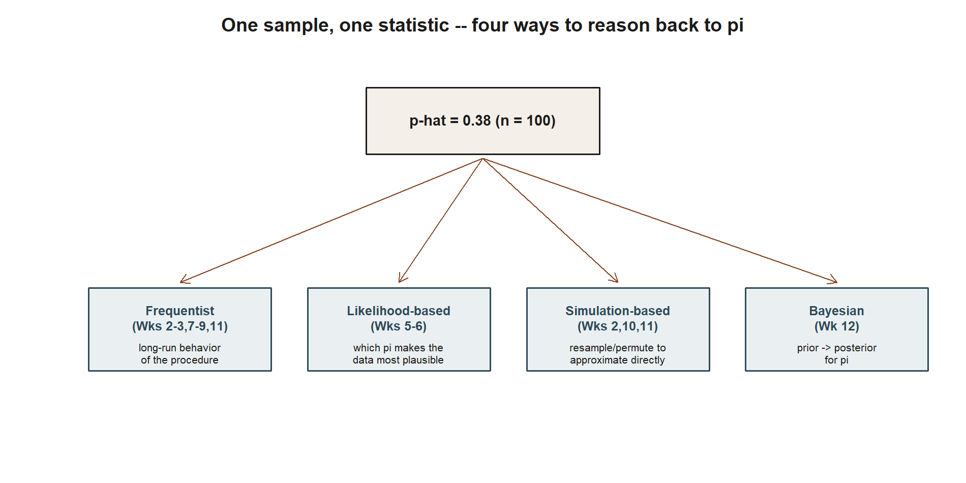
By Week 13, you will compare all four side by side on the exact same MAC Study usage-rate question, so this preview is worth remembering rather than memorizing in detail right now.
Worked examples
Worked example — MAC Study setup: naming the parameter, the sample, and the estimate
Symbolic setup. Let \(\pi\) denote the (unknown) population proportion of students in a large intro math course who use the MAC at least once in a given week. Suppose a sample of \(n\) such students is surveyed, and \(k\) of them report having used the MAC that week. The natural estimator for \(\pi\) is the sample proportion,
\[\hat{p} = \frac{k}{n}.\]
Numeric instance (MAC Study, full survey). The MAC Study’s full survey samples \(n = 100\) students, of whom \(k = 38\) report using the MAC at least once that week. Applying the estimator above,
\[\hat{p} = \frac{38}{100} = 0.38.\]
Here, \(\pi\) is the parameter (the true population usage rate — unknown, and not equal to 0.38 in general); \(\hat{p}\)-the-formula is the estimator; and \(0.38\) is this week’s particular estimate, produced by applying the estimator to this one sample. A different 100 students would almost surely give some other \(\hat{p}\) close to, but not exactly, 0.38 — sampling variability at work, quantified starting in Week 3.
Worked example — transfer: a pre-election poll (synthetic; illustrative numbers)
Setting (synthetic; illustrative numbers, not a real poll). A polling organization wants to estimate the proportion of registered voters in a city, call it \(\pi\), who currently support a particular candidate. It is not feasible to ask every registered voter, so the organization phones a random sample of voters instead.
Symbolic setup. Exactly as above, if \(n\) voters are sampled and \(k\) report supporting the candidate, the natural estimator for the population support rate \(\pi\) is
\[\hat{p} = \frac{k}{n}.\]
Numeric instance (synthetic). Suppose the polling organization reaches \(n = 400\) registered voters, and \(k = 212\) say they support the candidate. Then
\[\hat{p} = \frac{212}{400} = 0.53.\]
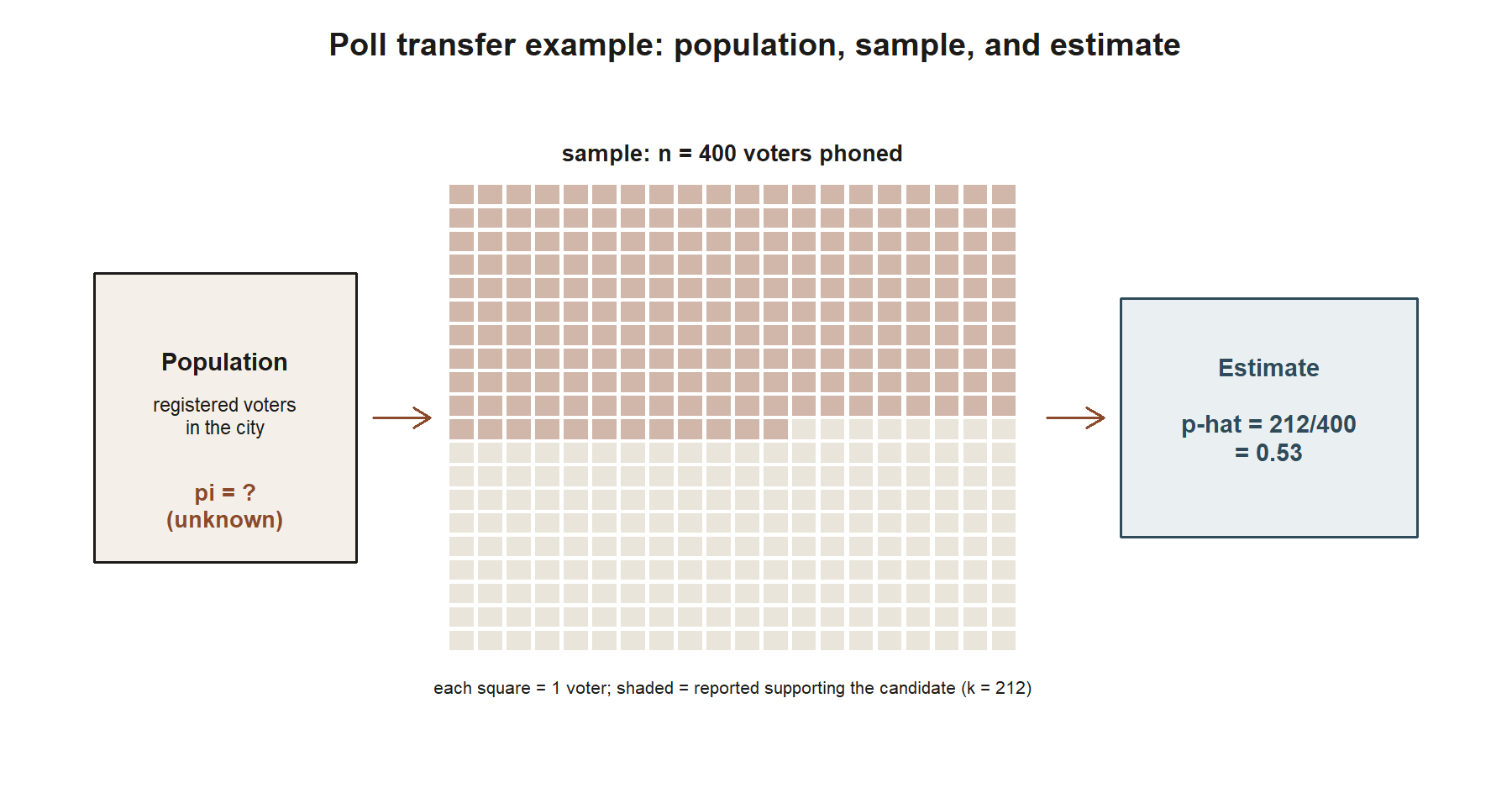
This \(0.53\), exactly like the MAC Study’s \(0.38\), is an estimate: one number, produced by one application of the sample-proportion estimator to one particular sample of voters. It is not the same thing as \(\pi\), the true (unknown, and in a real election, unknowable until the election is held) population support rate. A headline reporting “53% support” is really reporting \(\hat{p}\), and a responsible report must also convey how much \(\hat{p}\) could plausibly differ from \(\pi\) just from the luck of who was sampled — a margin of error, formalized later as a confidence interval (Week 3 onward, completing in Week 7). Notice the parallel to the MAC Study: different context, same inferential shape — an unknown population proportion, a sample proportion in hand, and a gap between the two that must be quantified rather than ignored.
A common mistake
A very common error at this stage is to treat the sample statistic as if it were the population parameter — saying “38% of students use the MAC” (a claim about the population) when what was actually established is “38% of these 100 surveyed students reported using the MAC” (a claim about the sample). The first statement asserts something about every student with no hedge at all; the second is the honest, narrower claim the data supports. Closing that gap responsibly — not by pretending it does not exist, and not by refusing to say anything at all — is the entire project of statistical inference, and it is why later weeks attach an explicit standard error, confidence interval, p-value, or posterior distribution to statistics like \(\hat{p}\) rather than reporting them as bare numbers.
A related mistake is assuming that because this sample gave \(\hat{p} = 0.38\), a repeat survey must give the same number. Sampling variability guarantees it generally will not; the rest of this course says precisely how much it should be expected to vary, rather than pretending it will not vary at all.
Low-stakes self-checks (ungraded)
These are practice prompts for your own study — ungraded, with no submission and no answer key.
- Write one sentence distinguishing a parameter from a statistic, and one distinguishing an estimator from an estimate.
- For the MAC Study’s visit-duration question, identify which symbol names the (unknown) population parameter and which symbol would name a statistic computed from a sample of visits.
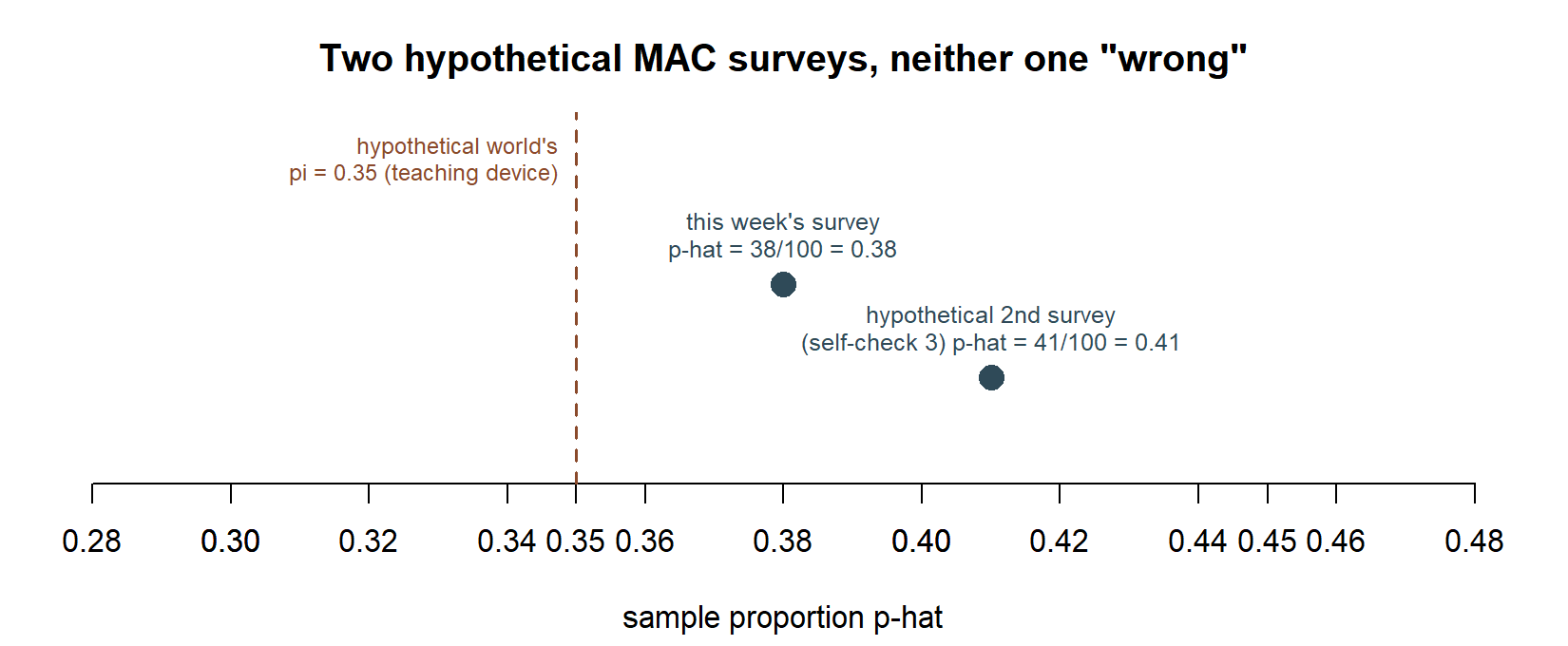
- Suppose a second, independent survey of 100 different students found \(k = 41\) MAC users instead of 38. Explain, without doing any calculation, why this outcome does not mean either survey made an error.
- Sketch what it would mean for the pre-election poll’s estimate \(\hat{p} = 0.53\) to be “close to” \(\pi\) versus “far from” \(\pi\).
- Name the four inferential traditions previewed this week, and, for each, write one phrase capturing what it treats as its central object.
Reading and source pointer
This week’s scope, sequence, and vocabulary are grounded in MIT OpenCourseWare 18.05, Introduction to Probability and Statistics, in its opening treatment of what statistical inference is and how it relates to probability and to descriptive statistics (https://ocw.mit.edu/courses/18-05-introduction-to-probability-and-statistics-spring-2022/). As an optional, lighter alternative pass over the same introductory ideas, you may also look at the opening statistical overview in Introduction to Modern Statistics (Çetinkaya-Rundel & Hardin), free at https://openintro-ims.netlify.app/ — not required, and not a source this course leans on, but a gentler first read if you want a second angle before returning to 18.05. These notes are the course’s own synthesis, grounded in but not copied from the sources.
Public vs. graded
These notes, the examples, and the practice here are public and ungraded — study material only. No graded prompts, answer keys, rubrics, point values, or due dates appear on this site. Graded inference checkpoints, quizzes, homework, labs, the midterm, the project, and the final live in Blackboard (the LMS), which is authoritative for due dates, submissions, and grades. If this page and Blackboard ever disagree, follow Blackboard.
Looking ahead
Week 2 puts the hypothetical “true” MAC Study world to work: it simulates drawing many samples from a known Normal(\(\mu = 48\), \(\sigma = 15\)) population, so you can see a sampling distribution take shape directly, before any formula is asserted for it. Week 3 then turns to standard errors for the real sample statistics (\(\bar{x}\) and \(\hat{p}\)) introduced today, building toward confidence intervals (Week 7) and hypothesis tests (Week 8) on the vocabulary set up this week.