Week 4 — Bias, variance, and mean squared error

Two ways an estimator can go wrong, and one number that combines them

Mathematical goal

Derive three quantities that describe how an estimator \(\hat\theta\) behaves across repeated sampling — \(\text{Bias}(\hat\theta)\), \(\text{Var}(\hat\theta)\), and \(\text{MSE}(\hat\theta)\) — and prove the decomposition \(\text{MSE}(\hat\theta) = \text{Var}(\hat\theta) + \text{Bias}(\hat\theta)^2\). Use that decomposition to explain two concrete facts this course needs later: why the sample variance divides by \(n-1\) rather than \(n\), and why an estimator with smaller variance can still be a poor choice if it carries too much bias.

The week question

An estimator \(\hat\theta\) is a formula applied to sample data, so it is itself a random variable — it takes a different value in every hypothetical repetition of the sample. Two separate things can go wrong with that randomness: \(\hat\theta\) can be systematically off-target on average (bias), and \(\hat\theta\) can bounce around a lot from sample to sample (variance). This week asks: how do we define each of these precisely, how do they combine into a single measure of estimator quality, and what does that measure teach us about two estimators this course will keep using — the sample variance and a “shrinkage” version of the sample mean?

Notation

Symbol	Meaning
\(\theta\)	the true (unknown) parameter value
\(\hat\theta\)	an estimator of \(\theta\) — a random variable, a function of the sample
\(E[\hat\theta]\)	the expected value of the estimator, averaged over all hypothetical samples
\(\text{Bias}(\hat\theta)\)	\(E[\hat\theta] - \theta\) — systematic over- or under-estimation
\(\text{Var}(\hat\theta)\)	\(E\big[(\hat\theta - E[\hat\theta])^2\big]\) — spread of \(\hat\theta\) around its own mean
\(\text{MSE}(\hat\theta)\)	\(E\big[(\hat\theta - \theta)^2\big]\) — average squared distance from the truth
\(n\)	sample size
\(\bar x\)	sample mean
\(s^2\)	sample variance, using the \(n-1\) divisor
\(\sigma^2\)	true population variance (hypothetical, teaching device only)
\(x_i\)	\(i\)-th observation in the sample

Conceptual setup

Every estimator this course has used so far — \(\bar x\) for \(\mu\), \(\hat p\) for \(\pi\) — is a random variable before the data are collected: it will take a different numerical value in each hypothetical repetition of the sampling process. Weeks 2 and 3 built the machinery to describe that randomness (the sampling distribution and its standard error). This week names two distinct ways an estimator’s sampling distribution can fail to sit where we want it, and shows how they combine into a single accuracy score.

Bias asks whether the center of the sampling distribution of \(\hat\theta\) sits at the true value \(\theta\):

\[ \text{Bias}(\hat\theta) = E[\hat\theta] - \theta. \]

If \(\text{Bias}(\hat\theta) = 0\), the estimator is called unbiased: it is correct on average, even though any single sample’s estimate can still miss. If \(\text{Bias}(\hat\theta) \neq 0\), the estimator is systematically too high or too low, no matter how large \(n\) gets (unless the bias itself shrinks with \(n\)).

Variance asks how far \(\hat\theta\) typically strays from its own average value, regardless of where that average sits:

\[ \text{Var}(\hat\theta) = E\big[(\hat\theta - E[\hat\theta])^2\big]. \]

A low-variance estimator is precise — repeated samples give similar answers — even if those answers are biased. A high-variance estimator is noisy from sample to sample, even if it is unbiased.

These are two independent failure modes. An estimator can be unbiased but noisy, biased but very precise, both, or neither. To compare estimators on a single scale, we need a quantity that folds both together. That quantity is the mean squared error:

\[ \text{MSE}(\hat\theta) = E\big[(\hat\theta - \theta)^2\big]. \]

MSE measures average squared distance from the true parameter value — the number we actually care about, since bias alone and variance alone each tell only half the story.

Deriving the decomposition. Insert and subtract \(E[\hat\theta]\) inside the square:

\[ \text{MSE}(\hat\theta) = E\big[(\hat\theta - \theta)^2\big] = E\Big[\big((\hat\theta - E[\hat\theta]) + (E[\hat\theta] - \theta)\big)^2\Big]. \]

Expand the square. Write \(A = \hat\theta - E[\hat\theta]\) (a random quantity with mean zero) and \(B = E[\hat\theta] - \theta\) (a fixed constant, since \(E[\hat\theta]\) and \(\theta\) are both non-random numbers):

\[ E\big[(A+B)^2\big] = E[A^2] + 2B\,E[A] + B^2. \]

Now evaluate each piece. First, \(E[A^2] = E\big[(\hat\theta - E[\hat\theta])^2\big] = \text{Var}(\hat\theta)\) by definition. Second, \(E[A] = E[\hat\theta - E[\hat\theta]] = E[\hat\theta] - E[\hat\theta] = 0\), so the middle term \(2B\,E[A]\) vanishes entirely. Third, \(B^2 = \big(E[\hat\theta] - \theta\big)^2 = \text{Bias}(\hat\theta)^2\). Putting the three pieces back together:

\[ \text{MSE}(\hat\theta) = \text{Var}(\hat\theta) + \text{Bias}(\hat\theta)^2. \]

This is the bias-variance decomposition. It says total average squared error splits cleanly into a variance piece (how noisy the estimator is) and a squared-bias piece (how systematically off-center it is), with no leftover cross term — the algebra above shows that cross term is exactly zero. One immediate consequence: for an unbiased estimator, \(\text{Bias}(\hat\theta) = 0\), so \(\text{MSE}(\hat\theta) = \text{Var}(\hat\theta)\) — mean squared error and variance coincide. That special case appears constantly: whenever this course calls \(\bar x\) or \(\hat p\) “unbiased,” their MSE is simply their variance, no bias term to track.

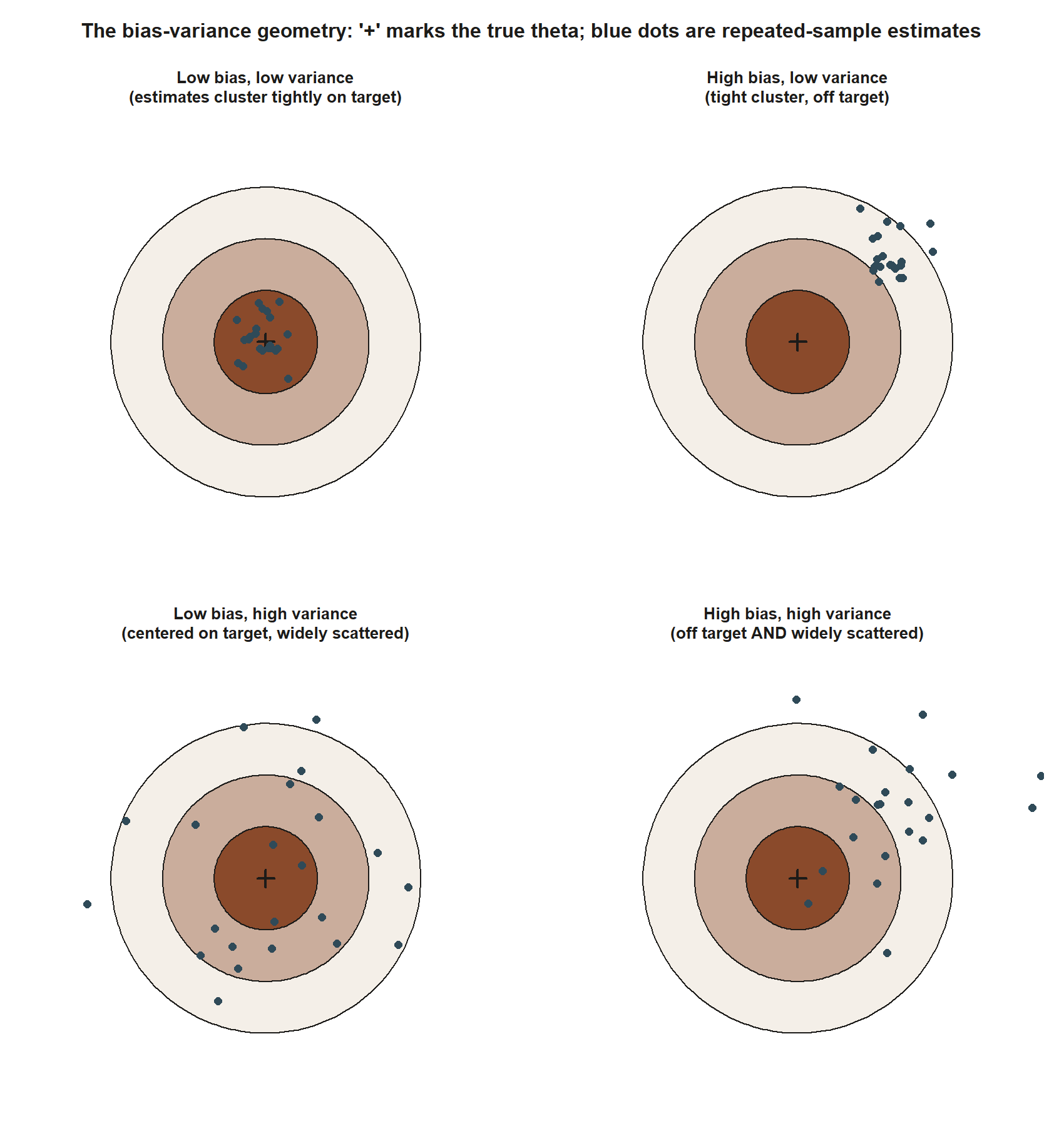
Before turning to numbers, it helps to see bias and variance as two independent, spatial failure modes rather than as two lines of algebra:

A 2 by 2 grid of four bullseye targets. Top-left, titled low bias low variance, shows points tightly clustered on the center cross. Top-right, titled high bias low variance, shows points tightly clustered but off to one side of the center cross. Bottom-left, titled low bias high variance, shows points widely scattered but centered on the cross. Bottom-right, titled high bias high variance, shows points widely scattered and off to one side of the cross. — Figure 1: **The bias-variance geometry (synthetic).** Four panels, one per combination: low bias/low variance (estimates cluster tightly on the true value), high bias/low variance (a tight cluster, off-target), low bias/high variance (centered on the true value but widely scattered), and high bias/high variance (off-target and widely scattered). The ‘+’ marks the true \(\theta\) in every panel; each blue dot is one hypothetical repeated-sample estimate.

What the figure shows (non-visual equivalent). Bias and variance are independent: an estimator’s repeated-sample estimates can be centered on the true value or systematically off it (bias), and separately can be tightly clustered or widely spread out (variance). The four panels walk all four combinations of “on-target vs. off-target” crossed with “tight vs. spread out.” MSE is the single number that folds both axes together, as the decomposition above shows algebraically. Synthetic instructional example; numbers are illustrative.

Worked example

MAC Study slice — why the sample variance divides by \(n-1\).

The sample variance formula students meet in intro stats is \(s^2 = \frac{1}{n-1}\sum_{i=1}^n (x_i - \bar x)^2\). The \(n-1\) divisor often looks arbitrary the first time it is seen. The bias-variance framework lets us show precisely why plugging in \(n\) instead would be the wrong choice — using the bias derivation, not simply asserting the result.

Consider the alternative statistic that divides by \(n\) instead of \(n-1\):

\[ \widetilde{S}^2 = \frac{1}{n}\sum_{i=1}^n (x_i - \bar x)^2. \]

A standard derivation (shown in 18.05, and stated here as the target this course builds toward) establishes that, when the \(x_i\) are drawn independently from a population with true variance \(\sigma^2\):

\[ E\big[\widetilde{S}^2\big] = \frac{n-1}{n}\,\sigma^2. \]

The intuition: \(\widetilde{S}^2\) measures spread around the sample mean \(\bar x\) rather than the true (unknown) mean \(\mu\), and \(\bar x\) is itself fit to the same data — it is always at least as close to the data points as the true \(\mu\) would be, so squared deviations from \(\bar x\) systematically understate squared deviations from \(\mu\). The factor \(\frac{n-1}{n}\) quantifies exactly how much that understatement is, on average.

Applying the bias definition directly:

\[ \text{Bias}\big(\widetilde{S}^2\big) = E\big[\widetilde{S}^2\big] - \sigma^2 = \frac{n-1}{n}\sigma^2 - \sigma^2 = \sigma^2\left(\frac{n-1}{n} - 1\right) = -\frac{\sigma^2}{n}. \]

So \(\widetilde{S}^2\) is always biased downward by \(\sigma^2/n\) — it systematically underestimates the true variance, and the size of that underestimate depends on both \(\sigma^2\) and \(n\).

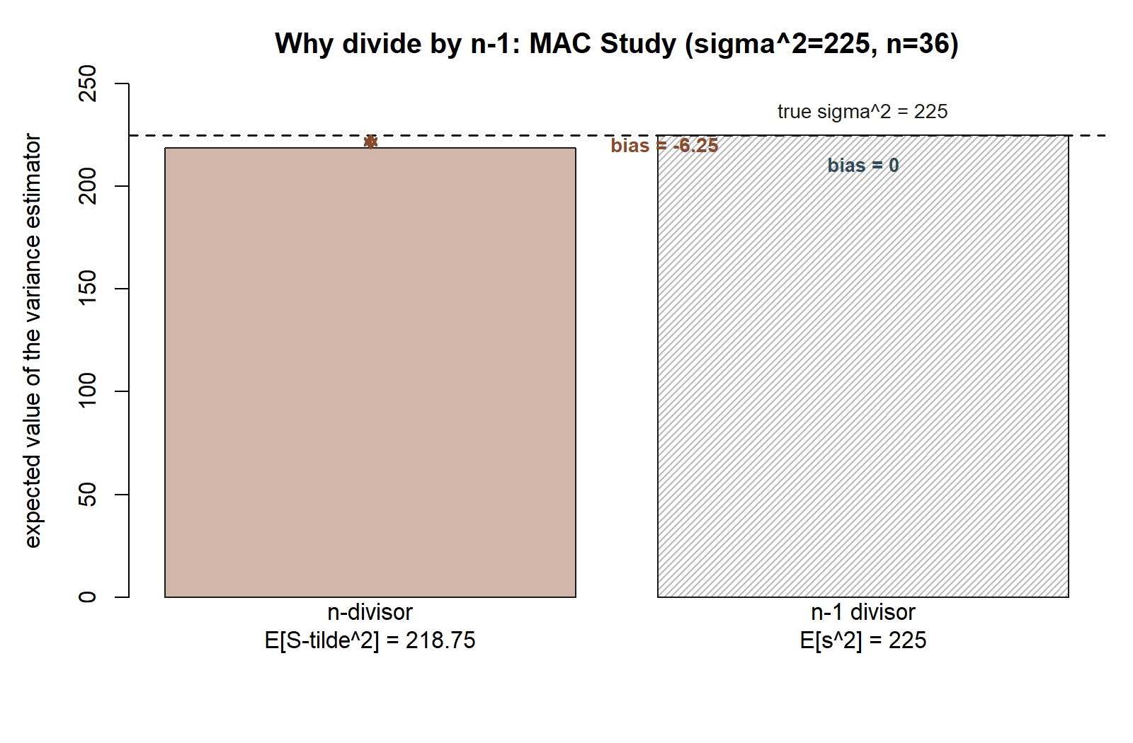
Now plug in this week’s numbers from the MAC Study’s hypothetical true world (Week 2’s stipulated backdrop: visit duration Normal(\(\mu = 48\), \(\sigma = 15\)), so \(\sigma^2 = 225\)), together with the sample size from the MAC Study’s visit-duration sample, \(n = 36\):

\[ E\big[\widetilde{S}^2\big] = \frac{n-1}{n}\sigma^2 = \frac{35}{36}(225). \]

Computing the fraction: \(\frac{35}{36}(225) = \frac{35 \times 225}{36} = \frac{7875}{36} = 218.75\).

\[ \text{Bias}\big(\widetilde{S}^2\big) = 218.75 - 225 = -6.25. \]

So if the population truly had variance \(225\) (a hypothetical fact never actually known to the analyst — flag this as a teaching device only, per this course’s convention), the \(n\)-divisor statistic would, on average across repeated samples of size 36, come in \(6.25\) units too low.

Why this motivates dividing by \(n-1\) instead. If we instead define \(s^2 = \frac{n}{n-1}\widetilde{S}^2 = \frac{1}{n-1}\sum_{i=1}^n (x_i - \bar x)^2\), then

\[ E[s^2] = \frac{n}{n-1}\,E\big[\widetilde{S}^2\big] = \frac{n}{n-1}\cdot\frac{n-1}{n}\sigma^2 = \sigma^2, \]

so \(\text{Bias}(s^2) = 0\) exactly, for any \(n\) and any \(\sigma^2\). Rescaling by \(\frac{n}{n-1}\) exactly cancels the bias found above. That is the precise, derived reason this course (and nearly every introductory course) defines the sample variance with an \(n-1\) divisor: it is the unique rescaling of \(\widetilde{S}^2\) that makes the estimator unbiased for \(\sigma^2\). This is also why the MAC Study’s sample SD is reported as \(s = 15.2\) minutes (Week 3) using this \(n-1\) convention, not the \(n\)-divisor alternative.

A two-bar chart. The left bar, labeled n-divisor, E of S-tilde-squared equals 218.75, reaches just below a dashed horizontal reference line marking the true sigma-squared of 225, with the gap labeled bias equals negative 6.25. The right bar, labeled n-1 divisor, E of s-squared equals 225, reaches exactly to the reference line, labeled bias equals 0. — Figure 2: **Why divide by \(n-1\): the MAC Study numbers, drawn (synthetic).** The \(n\)-divisor estimator \(\widetilde{S}^2\) comes in at 218.75 on average — 6.25 below the true \(\sigma^2=225\) (hatched reference line) — while the \(n-1\)-divisor estimator \(s^2\) lands exactly on 225.

What the figure shows (non-visual equivalent). For this course’s stipulated hypothetical world (\(\sigma^2=225\), \(n=36\)), the \(n\)-divisor variance estimator averages 218.75 across hypothetical repeated samples — 6.25 short of the true 225, a systematic downward bias that would persist no matter how many times the study were repeated. The \(n-1\)-divisor estimator averages exactly 225: zero bias, by construction. This is the same derivation as the algebra above, shown as two bar heights against one reference line instead of as equations. Synthetic instructional example; numbers are illustrative.

Transfer example (synthetic; seed set) — two ways to estimate widget-weight variance.

An assembly line packages widgets whose weights vary from unit to unit. Suppose, purely as a stipulated teaching fact for this synthetic example, the true population variance in widget weight is \(\sigma^2 = 4\) (grams\(^2\)), and a quality-control sample of \(n = 10\) widgets is weighed. Compare the two variance estimators at this sample size:

\[ E\big[\widetilde{S}^2\big] = \frac{n-1}{n}\sigma^2 = \frac{9}{10}(4) = 3.6, \qquad \text{Bias}\big(\widetilde{S}^2\big) = 3.6 - 4 = -0.4. \]

\[ E[s^2] = \sigma^2 = 4, \qquad \text{Bias}(s^2) = 0. \]

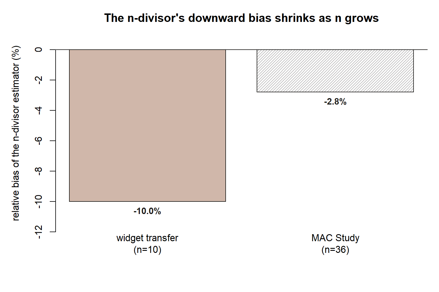
At this smaller sample size, the \(n\)-divisor estimator’s downward bias is proportionally larger relative to \(\sigma^2\) (\(-0.4/4 = -10\%\), versus \(-6.25/225 \approx -2.8\%\) in the MAC Study’s \(n=36\) case) — a reminder that this bias shrinks as \(n\) grows but never vanishes for the \(n\)-divisor version at any finite \(n\). The line’s quality-control analyst should report \(s^2\) (the \(n-1\) version), exactly as the MAC Study’s sample SD does.

MAC Study slice — the shrinkage estimator and why “unbiased” is not automatically better.

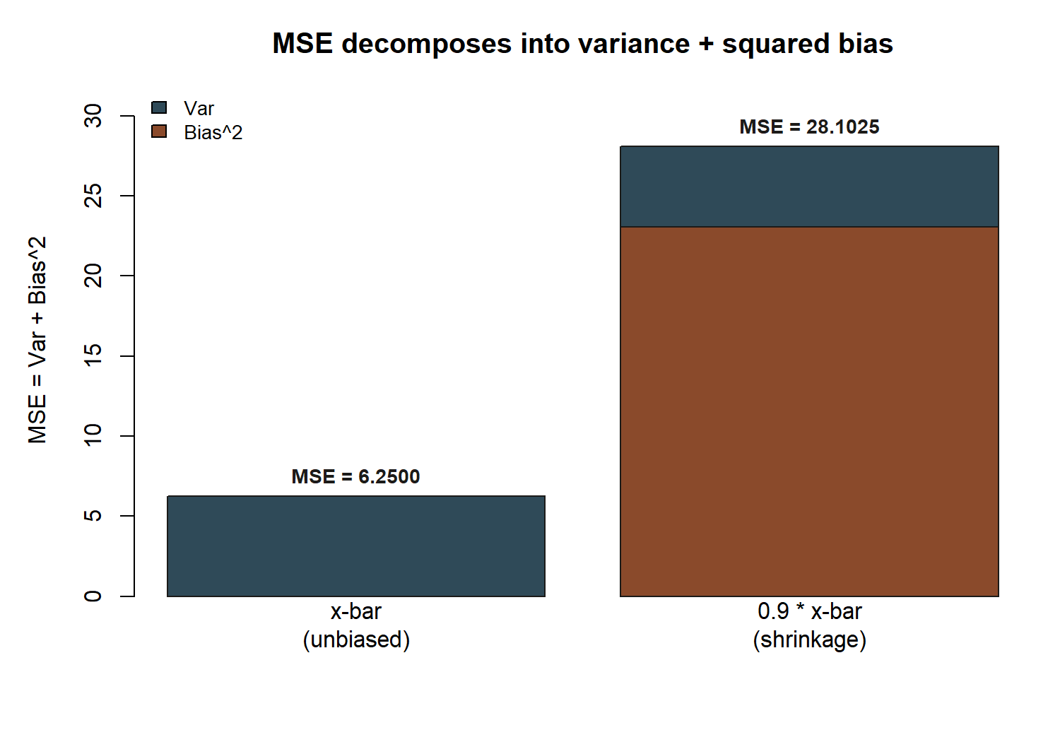
Now compare two estimators of the mean visit duration \(\mu\), using the MAC Study’s known-SE teaching simplification from Week 3: \(\bar x\) has \(\text{Var}(\bar x) = \text{SE}(\bar x)^2 = 2.5^2 = 6.25\), and (since \(\bar x\) is unbiased) \(\text{MSE}(\bar x) = \text{Var}(\bar x) = 6.25\).

Consider a shrinkage estimator \(\hat\theta = 0.9\,\bar x\) — one that deliberately pulls the sample mean toward zero by a fixed factor. Using this week’s hypothetical true world value \(\mu = 48\) (a stipulated true value for this teaching example only, exactly as flagged in Week 2):

\[ \text{Bias}(\hat\theta) = E[0.9\bar x] - \mu = 0.9\,E[\bar x] - \mu = 0.9(48) - 48 = 43.2 - 48 = -4.8. \]

For the variance, recall that multiplying a random variable by a constant \(c\) multiplies its variance by \(c^2\):

\[ \text{Var}(\hat\theta) = \text{Var}(0.9\bar x) = 0.9^2\,\text{Var}(\bar x) = 0.81(6.25) = 5.0625. \]

Now assemble the MSE using the decomposition derived above:

\[ \text{MSE}(\hat\theta) = \text{Var}(\hat\theta) + \text{Bias}(\hat\theta)^2 = 5.0625 + (-4.8)^2 = 5.0625 + 23.04 = 28.1025. \]

Compare directly to the unbiased \(\bar x\):

Estimator	Bias	Var	MSE
\(\bar x\) (unbiased)	\(0\)	\(6.25\)	\(6.25\)
\(\hat\theta = 0.9\bar x\) (shrinkage)	\(-4.8\)	\(5.0625\)	\(28.1025\)

The shrinkage estimator has smaller variance than \(\bar x\) (\(5.0625 < 6.25\)) — it is genuinely more precise, sample to sample. But its bias is large enough that its MSE is more than four times worse (\(28.1025\) vs. \(6.25\)). In this particular case, the variance reduction does not come close to paying for the bias it introduces.

A two-bar stacked chart. The left bar, labeled x-bar unbiased, is entirely one color reaching a total height of 6.25, all variance, no bias portion. The right bar, labeled 0.9 times x-bar shrinkage, is much taller at a total height of 28.1025, made of a large lower segment for squared bias, 23.04, topped by a smaller segment for variance, 5.0625. — Figure 4: **MSE decomposes into variance plus squared bias, drawn to scale (synthetic; this week’s own numbers).** \(\bar x\)’s entire MSE (6.25) is variance, since it is unbiased. The shrinkage estimator’s smaller variance segment (5.0625) is dwarfed by its squared-bias segment (23.04), pushing its total MSE to 28.1025.

What the figure shows (non-visual equivalent). Stacking each estimator’s variance and squared-bias segments on top of each other makes the decomposition \(\text{MSE}=\text{Var}+\text{Bias}^2\) visible as bar height rather than as an equation. \(\bar x\)’s bar is short and entirely variance (no bias segment, since it is unbiased). The shrinkage estimator’s bar is much taller — its smaller variance segment is real, but its large squared-bias segment more than cancels that advantage, exactly the target-diagram geometry above (high bias, low variance) applied to this week’s own numbers. Synthetic instructional example; numbers are illustrative.

A convention warning

“Lower variance” and “unbiased” are each, on their own, incomplete recommendations — only MSE weighs both at once. A very common mistake is to see that an estimator has smaller variance and conclude it must be “better,” without checking what that variance reduction cost in bias. The shrinkage example above is a worked counterexample: \(0.9\bar x\) is more precise than \(\bar x\) but far worse on the metric that actually matters, expected squared distance from the truth. The reverse mistake is just as common: assuming an unbiased estimator is automatically preferable to any biased alternative. It is not — an unbiased estimator with huge variance can have worse MSE than a slightly biased estimator with much smaller variance. This general pattern is often called the bias-variance tradeoff: some estimation strategies (shrinkage, regularization, and related ideas that recur in more advanced courses) deliberately accept a bit of bias to buy a larger reduction in variance, and whether that trade is worthwhile can only be judged by comparing MSE, not by inspecting bias or variance in isolation. In this course’s specific numbers, the trade was a bad one; the general lesson — always check MSE, not just one component — is the one to keep. A second, related warning already flagged in this course (§4 of the notation ledger): \(\text{Bias}(\hat\theta)\) is only computable when a true \(\theta\) is stipulated, which happens only in flagged hypothetical-truth teaching examples like this one — never treat a real sample’s estimate as if the true \(\mu\) were secretly known.

Practice (ungraded)

Self-check only — no submission, no key.

Using the same hypothetical true world (\(\sigma^2 = 225\)) but a sample size of \(n = 16\) instead of \(n = 36\), recompute \(E[\widetilde{S}^2]\) and \(\text{Bias}(\widetilde{S}^2)\) for the \(n\)-divisor variance estimator. Is the bias larger or smaller in magnitude than the \(n=36\) case, and does that match the general pattern described above?
Consider a different shrinkage factor, \(\hat\theta = 0.95\,\bar x\), with the same MAC Study true value \(\mu = 48\) and \(\text{Var}(\bar x) = 6.25\). Compute \(\text{Bias}(\hat\theta)\), \(\text{Var}(\hat\theta)\), and \(\text{MSE}(\hat\theta)\). Is this shrinkage factor closer to or farther from beating \(\bar x\)’s MSE of \(6.25\) than the \(0.9\) version was?
In your own words, explain why the middle “cross term” vanishes in the bias-variance decomposition derived above — what property of \(E[\hat\theta - E[\hat\theta]]\) makes that term exactly zero rather than merely small?

Reading and source pointer

MIT OCW 18.05 covers estimators, bias, and mean squared error, and this page’s scope, terminology, and notation level are grounded in that treatment. These notes are the course’s own synthesis, grounded in but not copied from the source.

Public vs. graded

These notes, the examples, and the practice here are public and ungraded — study material only. No graded prompts, answer keys, rubrics, point values, or due dates appear on this site. Graded inference checkpoints, quizzes, homework, labs, the midterm, the project, and the final live in Blackboard (the LMS), which is authoritative for due dates, submissions, and grades. If this page and Blackboard ever disagree, follow Blackboard.

Looking ahead

Week 5 turns from how good is an estimator to how do we find a good estimator in the first place, introducing the likelihood function as a way of ranking candidate parameter values against observed data. The bias/variance/MSE vocabulary from this week will resurface once maximum likelihood estimators are built in Week 6, and again whenever this course compares competing estimators later in the term.