Week 6 — Estimation: moments, bias, variance, and consistency

Where this week starts

Five weeks in, you can write down a model, derive the exact distribution of a statistic, and describe what happens to it as the sample grows. What you have not done is build anything. Week 5 gave you tools for describing an estimator somebody else proposed; this week you propose it, and a new problem arrives with the job. Two reasonable people can offer two different functions of the same data as estimators of the same \(\theta\), and point estimation is not finished until you can say which one to reach for and why.

The week has two halves. The first is construction: the method of moments is the oldest recipe in the subject and still the one worth meeting first, because it is purely mechanical. Write down what the model says the population moments are, set them equal to the sample moments, and solve. No likelihood, no optimization, often no more than a line of algebra. The second half is evaluation. Bias, variance, mean squared error and consistency are the words this course uses whenever it compares two procedures, and each should leave this page as a quantity you can compute rather than a slogan.

Keep the Week 1 discipline in view: everything below assumes the estimand is settled, and an estimator that is superb by every criterion here is worthless if it is aimed at the wrong target. By Thursday you should be able to take an unfamiliar one-parameter model, produce two candidate estimators, compute the bias and the variance of each in closed form, decide which has smaller mean squared error and at which sample sizes, and say why the winner is frequently the biased one.

Why this matters downstream

Here is the concrete stake. A calibration lab needs the upper limit of a rounding error modelled as uniform on \((0, \theta)\). One analyst reports twice the sample mean; another reports a small multiple of the largest reading. Both are unbiased, both look sensible, and at \(n = 40\) the first carries fourteen times the mean squared error of the second — the same error the second reaches from only ten readings. Three quarters of the sample has been paid for and thrown away.

The second stake is a habit of mind. A student who leaves this week believing that unbiasedness is the objective will reject shrinkage, penalized likelihood, and every Bayes estimator in the course on principle, and each of those is biased on purpose for the reason this page is about to derive. Week 9 builds posterior estimators that are biased by construction and often better; Week 12 exhibits a family where the biased estimator converges at a faster rate.

What you will be able to do

• Derive a method-of-moments estimator for a one- or two-parameter model, and state the conditions under which its moment equations have one usable root.
• Exhibit a sample whose method-of-moments estimate is logically impossible, and say what the recipe ignored.
• Compute bias, variance and mean squared error in closed form, and say which of the two terms drives the total.
• Decide whether one estimator dominates another: no larger mean squared error at every parameter value, and strictly smaller somewhere.
• Produce an unbiased estimator that is not consistent and a biased one that is.
• Read and design a Monte Carlo comparison, including the paired scheme that resolves a difference of under one percent.

Words worth owning

Term	What it means in this course
estimator	A function of the data alone, fixed before any data arrive; a random variable
estimate	The number that estimator takes on for the sample in hand
sampling distribution	The distribution of the estimator under repeated sampling from \(P_\theta\)
bias	\(\mathbb{E}_\theta[\hat\theta] - \theta\), computed separately at each \(\theta\)
mean squared error	\(\mathbb{E}_\theta[(\hat\theta - \theta)^2]\); the risk of \(\hat\theta\) under squared-error loss
consistency	\(\hat\theta_n \xrightarrow{p} \theta\) for every \(\theta\); a property of a whole sequence
dominates	Has mean squared error no larger at every \(\theta\), and strictly smaller at some \(\theta\)
relative efficiency	Ratio of two estimators’ mean squared errors at the same \(\theta\) and \(n\)

Building estimators out of moments

Let \(X_1, \dots, X_n\) be independent draws from \(f(x \mid \theta)\) with \(\theta \in \Theta \subseteq \mathbb{R}^p\). In words: every observation comes from the same distribution, the observations carry no information about each other beyond that, and the one unknown is \(\theta\). Write the population moments and the sample moments as

\[\mu_k(\theta) = \mathbb{E}_\theta[X^k], \qquad m_k = \frac{1}{n}\sum_{i=1}^{n} X_i^k, \qquad k = 1, 2, \dots\]

The population moment is a known function of the unknown parameter; the sample moment is a known function of the observed data. The method of moments declares them equal for as many \(k\) as there are unknowns and solves for \(\theta\).

The recipe, and why it usually works

Formally, \(\hat\theta_{\mathrm{MM}}\) is any solution in \(\Theta\) of the \(p\) equations \(\mu_k(\hat\theta_{\mathrm{MM}}) = m_k\), \(k = 1, \dots, p\). For one parameter that is one equation in one unknown, and it usually inverts by hand.

Three instances to keep at your fingertips. For Bernoulli(\(p\)), \(\mu_1 = p\), so \(\hat p = \bar{X}\). For Exponential with rate \(\lambda\), \(\mu_1 = 1/\lambda\), so \(\hat\lambda = 1/\bar{X}\). For Normal(\(\mu, \sigma^2\)) we need two equations, \(\mu_1 = \mu\) and \(\mu_2 = \sigma^2 + \mu^2\), whose root is \(\hat\mu = \bar{X}\) together with

\[\hat\sigma^2 = m_2 - \bar{X}^2 = \frac{1}{n}\sum_{i=1}^{n} X_i^2 - \bar{X}^2 = \frac{1}{n}\sum_{i=1}^{n} (X_i - \bar{X})^2 .\]

Confirm that last equality with a pencil; the same rearrangement returns in the second worked example.

Why should any of this be trustworthy? Because of the weak law of large numbers and the continuous mapping theorem, both from Week 5. If the moments exist, then \(m_k \xrightarrow{p} \mu_k(\theta)\) for each \(k\). Collect the first \(p\) moments into a map \(g : \Theta \to \mathbb{R}^p\) with \(g(\theta) = (\mu_1(\theta), \dots, \mu_p(\theta))\). If \(g\) is one-to-one with a continuous inverse on a neighbourhood of the true \(\theta\), then applying \(g^{-1}\) to the converging sample moments gives \(\hat\theta_{\mathrm{MM}} \xrightarrow{p} \theta\). So the recipe delivers consistency for free. That is a real virtue and also the beginning of the trouble, because consistency is a low bar.

Notice the three conditions. The moments must exist, which rules out the Cauchy at once and rules out heavy tails as soon as you reach for a second or third moment. The moment map must be invertible, an identifiability condition of exactly the Week 1 kind. And its inverse must be continuous, so that small wobbles in \(m_k\) do not produce jumps in \(\hat\theta\).

Three ways the recipe misbehaves

It is not unique. Nothing forces you to use the first \(p\) moments. For a Uniform(\(0, \theta\)) sample, matching the first moment gives \(2\bar{X}\), because \(\mathbb{E}_\theta[X] = \theta/2\). Matching the second moment instead gives \(\sqrt{3 m_2}\), because \(\mathbb{E}_\theta[X^2] = \theta^2/3\). Both are method-of-moments estimators in the same model, and they are different random variables. On the ten readings in the first worked example below they return \(3.30\) and \(3.310\); elsewhere they disagree by much more. A recipe with several outputs is not yet a principle, and Week 7 supplies the one that replaces it.

It can return an impossible estimate. Take three uniform observations on \((0, \theta)\) equal to \(0.1\), \(0.2\) and \(0.9\). Then \(\bar{x} = 0.4\) and the moment estimate is \(2\bar{x} = 0.8\). But we observed a value of \(0.9\), so \(\theta \ge 0.9\) with certainty. The estimate contradicts the data that produced it. Nothing prevents this, because the recipe never looks at the support of the density, only at averages. The same failure wears other clothes: a variance component estimated as a difference of two mean squares can come out negative, and a negative variance is outside \(\Theta\).

It ignores structure. Two moments summarize a density crudely. In the uniform model the largest observation says far more about \(\theta\) than the average does, and the recipe never consults it. Week 10 names what is being discarded — sufficiency — and Week 12 prices it.

What makes one estimator better than another

An estimator is a random variable, so comparing two estimators means comparing two distributions, and distributions do not come pre-ordered. To rank them we compress each sampling distribution to one number by choosing a loss. This course’s default is squared-error loss, whose risk is the mean squared error — a modelling decision like any other, and Week 9 shows what changes under absolute-error loss.

The decomposition that organizes everything

Fix \(\theta\) and write \(b(\theta) = \mathbb{E}_\theta[\hat\theta] - \theta\) for the bias. Then

\[\begin{aligned} \mathrm{MSE}_\theta(\hat\theta) &= \mathbb{E}_\theta\big[(\hat\theta - \theta)^2\big] \\ &= \mathbb{E}_\theta\Big[\big\{(\hat\theta - \mathbb{E}_\theta[\hat\theta]) + b(\theta)\big\}^2\Big] \\ &= \mathbb{E}_\theta\big[(\hat\theta - \mathbb{E}_\theta[\hat\theta])^2\big] + 2\, b(\theta)\, \mathbb{E}_\theta\big[\hat\theta - \mathbb{E}_\theta[\hat\theta]\big] + b(\theta)^2 \\ &= \operatorname{Var}_\theta(\hat\theta) + b(\theta)^2 . \end{aligned}\]

The middle term vanishes because \(b(\theta)\) is a constant once \(\theta\) is fixed and it multiplies the expectation of a centred variable. Every step is elementary; the identity it produces is the most-used one in estimation theory.

Squared bias and variance are the two pieces of mean squared error.

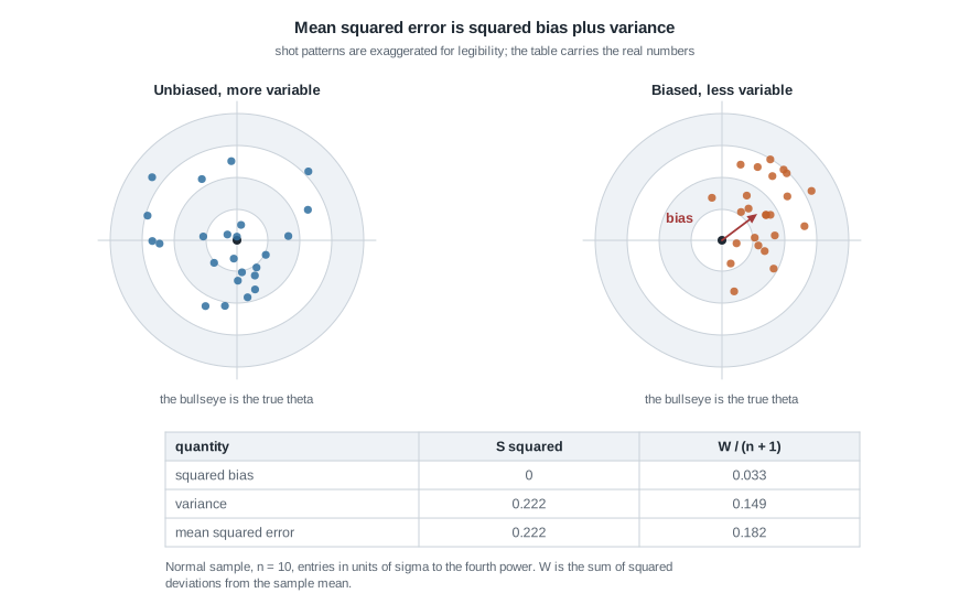
In the figure the left pattern is centred on the bullseye but sprays, the right is displaced but tight, and the mean squared error — the average squared distance from the bullseye — is won by the right. The table beneath carries the real numbers from the second worked example. Notice the subscript \(\theta\) on every symbol above: bias, variance and mean squared error are functions of the parameter, so two estimators can trade places as \(\theta\) moves. We say \(\hat\theta_A\) dominates \(\hat\theta_B\) when \(\mathrm{MSE}_\theta(\hat\theta_A) \le \mathrm{MSE}_\theta(\hat\theta_B)\) for every \(\theta \in \Theta\), with strict inequality somewhere; then \(\hat\theta_B\) is inadmissible under squared-error loss.

Now the general fact that both worked examples below turn out to be instances of. Suppose \(\hat\theta\) is unbiased with variance \(v = \operatorname{Var}_\theta(\hat\theta) \gt 0\), and shrink it toward zero by a factor \(c\). Then

\[\mathrm{MSE}_\theta(c\hat\theta) = c^2 v + (c-1)^2\theta^2 , \qquad \frac{d}{dc}\,\mathrm{MSE}_\theta(c\hat\theta)\Big|_{c=1} = 2v \gt 0 .\]

The derivative at \(c = 1\) is strictly positive, so moving \(c\) a little below one strictly reduces the mean squared error. Setting the derivative to zero gives the best multiple and its risk,

\[c^\ast = \frac{\theta^2}{v + \theta^2}, \qquad \mathrm{MSE}_\theta(c^\ast\hat\theta) = \frac{v\,\theta^2}{v + \theta^2} \lt v .\]

Read that as a sentence: no unbiased estimator with positive variance is ever the best multiple of itself. The catch is that \(c^\ast\) normally depends on \(\theta\), so \(c^\ast\hat\theta\) is not an estimator at all. One situation removes the catch. If the variance is proportional to the squared parameter, \(v = k\theta^2\) with \(k\) free of \(\theta\), then

\[c^\ast = \frac{1}{1+k}, \qquad \mathrm{MSE}_\theta(c^\ast\hat\theta) = \frac{k\,\theta^2}{1+k},\]

and \(c^\ast\) is a computable constant, so the shrunken estimator dominates the unbiased one everywhere. Any estimator whose standard deviation scales with \(\theta\) behaves this way, as does the normal variance, which is why both worked examples end with a biased winner.

Consistency is a separate promise

An estimator sequence \(\hat\theta_n\) is consistent for \(\theta\) if \(\hat\theta_n \xrightarrow{p} \theta\) under \(P_\theta\), for every \(\theta \in \Theta\). Note the shape: it is a claim about a sequence indexed by \(n\), and it must hold at every parameter value.

Chebyshev’s inequality gives the workhorse sufficient condition. For any \(\varepsilon \gt 0\),

\[P_\theta\big(|\hat\theta_n - \theta| \ge \varepsilon\big) \le \frac{\mathrm{MSE}_\theta(\hat\theta_n)}{\varepsilon^2},\]

so a vanishing mean squared error forces consistency; equivalently, it is enough that the bias and the variance both vanish. The condition is sufficient and not necessary. In a model where \(\bar{X}_n\) is consistent for \(\theta\), let \(\hat\theta_n\) equal \(\bar{X}_n\) with probability \(1 - 1/n\) and equal \(n\) otherwise, decided by an independent coin. It is consistent, since the bad event has probability \(1/n \to 0\), yet its mean squared error is at least \((n-\theta)^2/n\), which diverges.

More importantly, unbiasedness and consistency do not imply each other in either direction.

An unbiased estimator that never settles, beside a biased one that does.

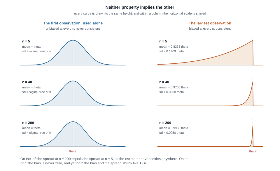
The left column is the estimator “use only the first observation” in a Normal(\(\theta, \sigma^2\)) model with \(\sigma^2\) known. Its expectation is \(\theta\) at every \(n\), so it is unbiased forever, and its sampling distribution stays Normal(\(\theta, \sigma^2\)) however much data you collect: it never settles, so it is not consistent. The right column is the sample maximum in a Uniform(\(0, \theta\)) model, whose mean \(n\theta/(n+1)\) sits below \(\theta\) at every finite \(n\). It is biased forever, but the bias \(-\theta/(n+1)\) and the standard deviation are the same order in \(n\), so both vanish and the estimator is consistent.

Worked example — the uniform upper endpoint

Setting. A calibration rig reports a rounding error the lab models as Uniform(\(0, \theta\)), with \(\theta\) unknown and the lower endpoint known to be zero. Ten independent readings, in micrometres, are

\[0.42,\; 1.83,\; 2.97,\; 0.15,\; 2.41,\; 1.06,\; 2.78,\; 0.63,\; 1.94,\; 2.31 .\]

Their total is \(16.50\), so \(\bar{x} = 1.650\), and the largest is \(x_{(10)} = 2.97\).

Step 1: the moments of the model. For \(X\) uniform on \((0, \theta)\) the density is \(1/\theta\) on that interval, so \(\mathbb{E}[X] = \theta/2\), \(\mathbb{E}[X^2] = \theta^2/3\), and therefore \(\operatorname{Var}(X) = \theta^2/3 - \theta^2/4 = \theta^2/12\).

Step 2: the moment estimator. Matching the first moment gives \(\hat\theta_1 = 2\bar{X}\), unbiased since \(\mathbb{E}_\theta[2\bar{X}] = \theta\), with

\[\operatorname{Var}_\theta(2\bar{X}) = 4\cdot\frac{\operatorname{Var}(X)}{n} = \frac{4\theta^2}{12 n} = \frac{\theta^2}{3n}, \qquad \mathrm{MSE}_\theta(2\bar{X}) = \frac{\theta^2}{3n}.\]

On these data the estimate is \(2(1.650) = 3.30\).

Step 3: the competitor built from the largest reading. Let \(M = X_{(n)}\). The maximum is at most \(t\) exactly when all \(n\) observations are, so

\[F_M(t) = P_\theta(M \le t) = \left(\frac{t}{\theta}\right)^{n}, \quad 0 \le t \le \theta, \qquad f_M(t) = \frac{n t^{n-1}}{\theta^{n}} .\]

Integrating gives the two moments we need,

\[\mathbb{E}_\theta[M] = \int_0^\theta t \cdot \frac{n t^{n-1}}{\theta^n}\,dt = \frac{n\theta}{n+1}, \qquad \mathbb{E}_\theta[M^2] = \int_0^\theta t^2 \cdot \frac{n t^{n-1}}{\theta^n}\,dt = \frac{n\theta^2}{n+2},\]

and subtracting the squared mean,

\[\operatorname{Var}_\theta(M) = \frac{n\theta^2}{n+2} - \frac{n^2\theta^2}{(n+1)^2} = \frac{n\theta^2\big\{(n+1)^2 - n(n+2)\big\}}{(n+2)(n+1)^2} = \frac{n\theta^2}{(n+2)(n+1)^2},\]

where the brace collapses because \((n+1)^2 - n(n+2) = n^2 + 2n + 1 - n^2 - 2n = 1\).

Step 4: correcting the bias. Since \(\mathbb{E}_\theta[M] = n\theta/(n+1)\), multiplying by \((n+1)/n\) produces an unbiased estimator \(\hat\theta_2 = \frac{n+1}{n}M\) with

\[\operatorname{Var}_\theta(\hat\theta_2) = \frac{(n+1)^2}{n^2}\cdot\frac{n\theta^2}{(n+2)(n+1)^2} = \frac{\theta^2}{n(n+2)} = \mathrm{MSE}_\theta(\hat\theta_2).\]

On these data the estimate is \(\tfrac{11}{10}(2.97) = 3.267\).

Step 5: compare the two unbiased estimators. Both are exactly unbiased, so the comparison is purely a variance comparison, and the ratio is

\[\frac{\mathrm{MSE}_\theta(2\bar{X})}{\mathrm{MSE}_\theta(\hat\theta_2)} = \frac{\theta^2/(3n)}{\theta^2/(n(n+2))} = \frac{n+2}{3}.\]

At \(n = 10\) the ratio is four and at \(n = 40\) it is fourteen. At \(n = 1\) it is one, as it must be: with a single observation \(2\bar{X}\) and \(\frac{n+1}{n}X_{(n)}\) are the same random variable \(2X_1\). That agreement is a free audit of the derivation, and exactly the check to run before believing algebra.

Two unbiased estimators of the same theta, drawn on one horizontal scale.

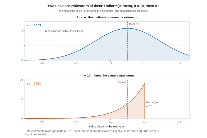
The figure draws both exact sampling distributions at \(n = 10\), \(\theta = 1\). They average to the same place and look nothing alike: the moment estimator is nearly symmetric, while the corrected maximum is sharply left-skewed with a hard edge at \(1.1\theta\), since \(M\) can never exceed \(\theta\). Only the second moment of that picture reaches the mean squared error.

Step 6: let the shrinkage lemma finish the job. \(\hat\theta_2\) is unbiased with variance \(v = \theta^2/(n(n+2))\), which is \(k\theta^2\) with \(k = 1/(n(n+2))\) free of \(\theta\). The lemma from the concept section therefore applies with a computable constant:

\[c^\ast = \frac{1}{1+k} = \frac{n(n+2)}{(n+1)^2}, \qquad c^\ast\hat\theta_2 = \frac{n(n+2)}{(n+1)^2}\cdot\frac{n+1}{n}M = \frac{n+2}{n+1}\,M .\]

Its mean squared error is \(k\theta^2/(1+k) = \theta^2/\{n(n+2)+1\} = \theta^2/(n+1)^2\), and its bias is \(-\theta/(n+1)^2\). On these data the estimate is \(\tfrac{12}{11}(2.97) = 3.24\).

Estimator	Bias	Mean squared error	MSE at \(n = 10\)	Estimate
\(2\bar{X}\)	\(0\)	\(\theta^2/(3n)\)	\(0.03333\,\theta^2\)	\(3.30\)
\(M = X_{(n)}\)	\(-\theta/(n+1)\)	\(2\theta^2/\{(n+1)(n+2)\}\)	\(0.01515\,\theta^2\)	\(2.97\)
\(\frac{n+1}{n}M\)	\(0\)	\(\theta^2/\{n(n+2)\}\)	\(0.00833\,\theta^2\)	\(3.267\)
\(\frac{n+2}{n+1}M\)	\(-\theta/(n+1)^2\)	\(\theta^2/(n+1)^2\)	\(0.00826\,\theta^2\)	\(3.24\)

Mean squared error against sample size, on logarithmic axes.

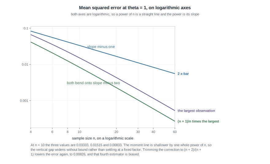
The second row is worth re-deriving: \(\mathrm{MSE}(M) = \operatorname{Var}(M) + \theta^2/(n+1)^2\), and over the common denominator \(n/\{(n+2)(n+1)^2\} + 1/(n+1)^2 = 2/\{(n+1)(n+2)\}\). The figure plots the first three rows with both axes logarithmic, and that choice is the whole point of the picture: a pure power \(c\,n^{-r}\) has \(\log(\mathrm{MSE}) = \log c - r \log n\), a straight line in \(\log n\) whose slope is exactly the rate \(-r\). The uneven tick spacing along the bottom is the visual signature that the horizontal axis has been logged too; on a plot with \(n\) spaced evenly, none of these graphs would be straight and no slope would be readable. The moment estimator’s error is the pure power \(1/(3n)\), so its graph is exactly straight with slope \(-1\), the shallower of the two rates on show. The two maximum-based errors, \(2/\{(n+1)(n+2)\}\) and \(1/\{n(n+2)\}\), are not quite pure powers — each is a power times a factor tending to one — so their graphs bend gently and settle onto slope \(-2\): twice as steep, an error shrinking one whole power of \(n\) faster. Read the vertical gap rather than the heights. It widens without bound, because a difference of rate, unlike a difference in the constant out front, is not a fixed handicap. Week 12 explains why the usual information bound has nothing to say about any of this.

What this assumed. Everything above used the uniform model exactly, including the known lower endpoint of zero. The maximum-based estimators are superb under that model and fragile away from it. Inflate one reading by \(\delta\): if it is the largest, \(\frac{n+1}{n}M\) moves by \(1.1\delta\) at \(n = 10\), while \(2\bar{X}\) moves by only \(\delta/5\). Efficiency under a model and robustness to a wrong model are different goods, and Week 14 prices the trade.

The same reasoning, transferred

Run the same ledger on a Poisson(\(\lambda\)) sample, where the mean and the variance are both \(\lambda\). Matching the first moment gives \(\hat\lambda_1 = \bar{X}\) at once. Matching the second is worth doing slowly, because this is where a plausible-sounding sentence goes wrong. The definition at the top of this page sets a population raw moment equal to a sample raw moment, and \(\mathbb{E}_\lambda[X^2] = \operatorname{Var}(X) + \{\mathbb{E}_\lambda[X]\}^2 = \lambda + \lambda^2\), so the second moment equation is the quadratic \(\hat\lambda + \hat\lambda^2 = m_2\), whose positive root is

\[\hat\lambda_2 = \frac{\sqrt{1 + 4m_2} - 1}{2} .\]

This is the same manoeuvre the uniform model asked for two sections above, where \(\mathbb{E}[X^2] = \theta^2/3\) gave \(\sqrt{3m_2}\); here the population second moment is quadratic in the parameter rather than a perfect square, so inverting it takes the quadratic formula. Non-uniqueness bites again: \(\hat\lambda_1\) and \(\hat\lambda_2\) are different random variables solving the recipe in one model. The second is consistent, by the continuous-mapping argument above, and its exact expectation is not available in closed form — which is itself the lesson that the recipe hands you consistency cheaply and finite-sample properties not at all.

What \(\hat\lambda_2\) is not is the sample variance. Substituting the first equation into the second instead of solving it outright gives the plug-in \(m_2 - \bar{X}^2 = \frac{1}{n}\sum_i (X_i - \bar{X})^2 = \frac{n-1}{n}S^2\) — exactly the rearrangement you were asked to confirm with a pencil for the normal, and note the divisor \(n\) rather than \(n-1\). Its expectation is \((n-1)\lambda/n\), low by \(\lambda/n\). So neither route produces the unbiased \(S^2\), and calling \(S^2\) “the second moment estimator” here would contradict the definition this page started from.

Compare \(\bar{X}\) instead with the competitor that the model identity \(\operatorname{Var}(X) = \lambda\) suggests to any working statistician: the unbiased \(S^2\), which estimates \(\lambda\) because in this model the variance is the parameter. Both estimators are exactly unbiased, so this comparison, like the uniform one, is purely a comparison of variances.

The first variance is immediate, \(\operatorname{Var}_\lambda(\bar{X}) = \lambda/n\). The second needs the standard identity \(\operatorname{Var}(S^2) = \frac{1}{n}\{\mu_4 - \frac{n-3}{n-1}\sigma^4\}\), where \(\mu_4\) is the fourth central moment. For the Poisson every cumulant equals \(\lambda\), so \(\mu_4 = \kappa_4 + 3\kappa_2^2 = \lambda + 3\lambda^2\), and

\[\operatorname{Var}_\lambda(S^2) = \frac{\lambda}{n} + \frac{\lambda^2}{n}\left\{3 - \frac{n-3}{n-1}\right\} = \frac{\lambda}{n} + \frac{\lambda^2}{n}\cdot\frac{2n}{n-1} = \frac{\lambda}{n} + \frac{2\lambda^2}{n-1}.\]

So \(\bar{X}\) wins by exactly \(2\lambda^2/(n-1)\) at every \(\lambda\) and every \(n \ge 2\). At \(\lambda = 4\) and \(n = 25\) the two variances are \(0.160\) and \(1.493\), a relative efficiency of about eleven percent for \(S^2\).

The moment plug-in \(\frac{n-1}{n}S^2\) is no rescue either. It is biased, so it must be judged on mean squared error rather than variance, and that error is \(\big(\frac{n-1}{n}\big)^2 \operatorname{Var}_\lambda(S^2) + \lambda^2/n^2\), which at the same \(\lambda = 4\) and \(n = 25\) comes to \(0.9216(1.493) + 0.0256 = 1.402\) against \(0.160\) for \(\bar{X}\). Shrinking a very noisy estimator toward zero shaves a little off a large error and leaves it large; the shrinkage lemma promises an improvement over the estimator you started from, never a competitive one.

What stayed the same is the procedure: write down the population moments, match them, notice that the recipe again offers more than one root, then take expectations and variances and compare at a common \(n\). What changed is the verdict. In the uniform model the mean-based estimator lost badly to one built from an extreme order statistic; here it wins by a factor of nine, since \(1.493/0.160 = 9.3\). There is no rule of thumb behind these examples — the arithmetic is the rule. Week 10 notes that \(\bar{X}\) is a function of the sufficient statistic \(\sum_i X_i\) while \(S^2\) is not, and Week 11 makes that the reason the contest was never close.

Second worked example — shrinking the sample variance

Setting. A filling line is checked by weighing ten cartons; the weights, in grams, are modelled as independent Normal(\(\mu, \sigma^2\)), both parameters unknown. They are

\[17.4,\; 18.4,\; 18.4,\; 19.4,\; 20.4,\; 20.4,\; 21.4,\; 22.4,\; 22.4,\; 23.4 .\]

They total \(204.0\), so \(\bar{x} = 20.40\), and the deviations from the mean are \(-3, -2, -2, -1, 0, 0, 1, 2, 2, 3\), whose squares total \(W = 36.0\).

Step 1: what Week 4 already gives. Writing \(W = \sum_i (X_i - \bar{X})^2\), normal theory gives \(W/\sigma^2 \sim \chi^2_{n-1}\). A chi-square with \(m\) degrees of freedom has mean \(m\) and variance \(2m\), so with \(m = n-1\),

\[\mathbb{E}[W] = (n-1)\sigma^2, \qquad \operatorname{Var}(W) = 2(n-1)\sigma^4 .\]

Step 2: study one whole family at once. Restrict attention for the moment to the scale family \(\hat\sigma^2_c = cW\) with \(c \gt 0\) — the estimators that use the data only through the sum of squared deviations — and let the mean squared error pick \(c\) within that family:

\[\mathrm{MSE}(cW) = c^2 \operatorname{Var}(W) + \big\{c\,\mathbb{E}[W] - \sigma^2\big\}^2 = \sigma^4\Big[2(n-1)c^2 + \big\{(n-1)c - 1\big\}^2\Big].\]

Step 3: minimize. Write \(m = n-1\) and differentiate the bracket with respect to \(c\):

\[4mc + 2m(mc - 1) = 0 \;\Longrightarrow\; 2c + (mc - 1) = 0 \;\Longrightarrow\; c^\ast = \frac{1}{m+2} = \frac{1}{n+1}.\]

The bracket is a strictly convex quadratic in \(c\), its \(c^2\) coefficient being \(m^2 + 2m \gt 0\), so the stationary point is the minimum, and substituting it back gives \(\mathrm{MSE}(W/(n+1)) = 2\sigma^4/(n+1)\). State the conclusion at exactly its true strength: \(W/(n+1)\) is the minimum-error member of the family \(\{cW\}\). Nothing here says it is the best estimator of \(\sigma^2\) in any wider sense, and Step 5 will not need it to be.

Step 4: name the three familiar members. Taking \(c = 1/(n-1)\) gives the unbiased \(S^2\); \(c = 1/n\) gives the maximum likelihood estimator Week 7 will derive; \(c = 1/(n+1)\) gives the minimum-error member, biased downward by \(-2\sigma^2/(n+1)\).

Estimator	Bias	Mean squared error	Value at \(n = 10\), \(W = 36\)
\(S^2 = W/(n-1)\)	\(0\)	\(2\sigma^4/(n-1) = 0.2222\,\sigma^4\)	\(4.000\)
\(W/n\)	\(-\sigma^2/n\)	\((2n-1)\sigma^4/n^2 = 0.1900\,\sigma^4\)	\(3.600\)
\(W/(n+1)\)	\(-2\sigma^2/(n+1)\)	\(2\sigma^4/(n+1) = 0.1818\,\sigma^4\)	\(3.273\)

Step 5: read the verdict honestly. The ordering \(0.1818 \lt 0.1900 \lt 0.2222\) holds at every \((\mu, \sigma^2)\), since all three errors are the same constant times \(\sigma^4\). So \(W/(n+1)\) dominates \(S^2\), and \(S^2\) — the estimator every software package reports — is inadmissible under squared-error loss. It is the shrinkage lemma again: \(S^2\) is unbiased with variance \(k(\sigma^2)^2\) for \(k = 2/(n-1)\), so \(c^\ast = 1/(1+k) = (n-1)/(n+1)\) and \(c^\ast S^2 = W/(n+1)\).

That is not a recommendation to stop reporting \(S^2\). At \(n = 10\) the shrunken estimator runs eighteen percent low in expectation, a real distortion if the number is read as a variance rather than fed into a squared-error decision, and the optimal \(c\) leaned on normality through \(\operatorname{Var}(W) = 2(n-1)\sigma^4\). Note also what fails to discriminate: all three are consistent, so consistency cannot choose among them.

And \(W/(n+1)\) is not itself the bottom of anything. Step 2 fenced off a one-parameter family and Step 3 searched inside the fence; leaving the fence changes the picture. Note that \(W + n\bar{X}^2 = \sum_i X_i^2\), a sum of squares about the known value zero rather than about \(\bar{X}\). Were \(\mu\) actually zero, that sum over \(\sigma^2\) would be \(\chi^2_n\) — one more degree of freedom than \(W\) carries — and Steps 2 and 3 rerun with \(m = n\) would name \(\sum_i X_i^2/(n+2)\) as the minimum-error multiple of it. Stein’s estimator \(\min\{W/(n+1),\, (W + n\bar{X}^2)/(n+2)\}\) reports whichever of those two is the smaller, and has uniformly smaller mean squared error than \(W/(n+1)\) at every \((\mu, \sigma^2)\), including \(\mu \ne 0\). It is not a multiple of \(W\), so it lives outside the family Step 2 fixed, and its existence makes \(W/(n+1)\) inadmissible in turn. That is the honest shape of every verdict on this page: a domination claim is a statement about the estimators actually put side by side, never a proof that no further candidate exists.

Checking the algebra with a simulation

Proof and computation are complementary evidence here, so confirm the table. The block below forms all four uniform estimators from the same draws and compares simulated error against the closed forms.

set.seed(75063)
theta <- 1
n     <- 10
reps  <- 200000

sim <- t(replicate(reps, {
  x <- runif(n, 0, theta)
  c(mom = 2 * mean(x), mx = max(x))
}))

est <- cbind(mom      = sim[, "mom"],
             raw_max  = sim[, "mx"],
             unbiased = (n + 1) / n * sim[, "mx"],
             min_mse  = (n + 2) / (n + 1) * sim[, "mx"])

round(colMeans(est) - theta, 5)        # simulated bias
round(colMeans((est - theta)^2), 6)    # simulated mean squared error
round(c(1 / (3 * n),
        2 / ((n + 1) * (n + 2)),
        1 / (n * (n + 2)),
        1 / (n + 1)^2), 6)             # the closed forms derived above

Two features of the design matter. All three maximum-based estimators are built from the same stored maxima, so the comparison is paired: the difference in squared error on each replicate is a fixed function of one random quantity, and a gap of well under one percent is resolved that two independent runs of this length would leave in the noise. And a simulation confirms rather than proves. Agreement at \(\theta = 1\) and \(n = 10\) is consistent with an algebra error that cancels there, which is why the \(n = 1\) check in Step 5 is worth as much as the Monte Carlo run.

The misreading to avoid

Here is the sentence graduate students write this week, almost verbatim: “Since \(\frac{n+1}{n}X_{(n)}\) is unbiased and \(\frac{n+2}{n+1}X_{(n)}\) is not, the first is the estimator to use.” Or: “\(S^2\) is right for \(\sigma^2\) because it is unbiased.” Unbiasedness is being treated as the objective rather than as one coordinate of a two-coordinate description.

Four things are wrong with that. First, the arithmetic on this page refutes it. The biased \(\frac{n+2}{n+1}X_{(n)}\) has error \(\theta^2/(n+1)^2\) against \(\theta^2/\{n(n+2)\}\) for the unbiased competitor, and \((n+1)^2 = n(n+2) + 1\) exceeds \(n(n+2)\), so the biased estimator is strictly better at every \(\theta \gt 0\) and every \(n\). Likewise \(W/(n+1)\) dominates \(S^2\). Domination is not a matter of preference.

Second, the shrinkage lemma says this is no accident. An unbiased estimator with positive variance sits at \(c = 1\) on a curve whose derivative there is \(2v \gt 0\), so it is never at the bottom of its own family. Unbiasedness places you at a point guaranteed not to be optimal.

Third, unbiasedness is not preserved by reparameterization. \(S^2\) is unbiased for \(\sigma^2\), but the square root is strictly concave, so Jensen’s inequality gives \(\mathbb{E}[S] \lt \sigma\) whenever \(S^2\) is non-degenerate. For the normal at \(n = 10\), \(\mathbb{E}[S] = \sigma\sqrt{2/9}\,\Gamma(5)/\Gamma(4.5) \approx 0.9727\,\sigma\), low by nearly three percent. The same procedure is “unbiased” on the variance scale and biased on the standard deviation scale, and a property that flips when you relabel the parameter cannot by itself be the goal.

Fourth, unbiased estimators can be ridiculous. Take one observation \(X \sim\) Poisson(\(\lambda\)) with target \(e^{-2\lambda}\), a number in \((0, 1)\). Then

\[\mathbb{E}_\lambda\big[(-1)^X\big] = \sum_{x=0}^{\infty} (-1)^x \frac{e^{-\lambda}\lambda^x}{x!} = e^{-\lambda}\sum_{x=0}^{\infty}\frac{(-\lambda)^x}{x!} = e^{-\lambda}e^{-\lambda} = e^{-2\lambda},\]

so \((-1)^X\) is unbiased. It also takes only the values \(+1\) and \(-1\): one lies outside the range of the target, and the other is a supremum the target only approaches. Unbiasedness has been satisfied to the letter and the estimator is useless.

The opposite overcorrection is its own error, though. Restricting attention to unbiased estimators is what makes an optimality theory possible: without some restriction the constant \(\hat\theta \equiv \theta_0\) has zero variance and beats everything near \(\theta_0\). Week 11 shows what the unbiased class buys — Rao-Blackwell improvement, completeness, a genuinely best unbiased estimator — and says just as plainly that the class is not sacred. Treat unbiasedness as a modelling choice you can defend.

Practice on your own

For your own checking, not for submission. Attempt them before looking anything up.

1. Two-endpoint moments. For a Uniform(\(a, b\)) sample with both endpoints unknown, derive the moment estimators from the first two moments; you should reach \(\hat a = \bar{X} - \sqrt{3\hat\sigma^2}\) and \(\hat b = \bar{X} + \sqrt{3\hat\sigma^2}\) with \(\hat\sigma^2 = m_2 - \bar{X}^2\). Then build a small sample for which \(\hat a\) exceeds the smallest observation, and say what the recipe failed to consult.
2. Chebyshev in both directions. Prove that \(\mathrm{MSE}_\theta(\hat\theta_n) \to 0\) implies consistency, then verify the converse fails using the coin-flip construction above and find how fast its error diverges.
3. A counterexample hunt. Find two estimators of a normal mean whose risk curves cross, so neither dominates. Start from \(\bar{X}\) and \(c\bar{X}\) with fixed \(c \lt 1\), plot both risks against \(\mu\), and identify the interval of \(\mu\) where shrinkage wins.
4. Simulation at the extremes. Rerun the R block at \(n = 3\) and at \(n = 100\), and check the simulated ratio of the two unbiased errors against the predicted \((n+2)/3\). Explain why the maximum-based estimator’s simulated distribution looks less normal as \(n\) grows, not more.
5. Audit a plausible wrong argument. Someone writes: “Because \(\mathbb{E}[X_{(n)}] = \frac{n}{n+1} \theta\) and \(\frac{n}{n+1} \to 1\), the sample maximum is asymptotically unbiased, so for large \(n\) its mean squared error is the same as that of the corrected \(\frac{n+1}{n}X_{(n)}\).” Locate the false step and compute the limiting ratio of the two errors. It is not one.

Where to read more

• MIT OpenCourseWare 18.655, Mathematical Statistics — the decision-theoretic framing of loss, risk and domination that this page uses informally.
• MIT OpenCourseWare 18.650, Statistics for Applications — the method of moments and estimator comparison at a gentler pace.
• Penn State STAT 414 — a refresher on order statistics and moments of standard families, if Step 3 moved too fast.
• The R Project — the environment the simulation block runs in.
• Hogg, McKean and Craig chapter 7 covers this material in the conventional order; the course notes remain the primary source and nothing needs to be purchased.
• Course pages: the syllabus carries the course policies, and the resources page collects the computing setup.

Where this goes next

Next week replaces the recipe with a principle. The method of moments works because averages converge, which says nothing about which function of the data to average. Likelihood asks a sharper question — which parameter value makes the data actually observed most probable — and answers it with one construction that fits every model in this course. Its estimator in the uniform model turns out to be \(X_{(n)}\) itself, reached without any moment matching, and the curvature of the log-likelihood predicts variances of the kind you computed by hand here. Read Week 7 with this week’s table beside you, and notice which of the four uniform estimators likelihood hands you and which it does not. If the convergence language above felt thin, Week 5 repairs it.

The Bayesian thread picks up here too. A posterior mean is a weighted average of a prior mean and the data, so it is shrunken by construction, and the lemma on this page already predicts that it will often beat the unbiased estimator on mean squared error. Week 9 draws those risk curves. Return to the notes index for the full sequence.