Probability as the language of plausibility, and what changes when evidence arrives
The week question
If you are not sure about something — say, what fraction of students at this campus bike to class — how should seeing a little bit of data change your mind?
That is the whole course in one sentence, and it is the only question we ask this week. We are not going to compute anything heavy. We are going to build the habit of mind that everything else rests on: holding uncertainty honestly, and then moving it in a disciplined way when evidence shows up.
Where we are and why this matters
This is the first week, so there is no prior week to bridge from — but that is fitting, because “what should I believe before I have data, and how should data revise it?” is exactly where Bayesian thinking begins. You are standing at the start of a single, coherent line of reasoning that the rest of the term will sharpen.
Most statistics you have met before starts from data and asks a yes/no question about a fixed-but-unknown number: reject or fail to reject. Bayesian thinking reorganizes that. It treats the unknown number itself as something you can be more or less sure about, describes that uncertainty with a probability distribution, and then updates the distribution as data arrive. The payoff is enormous and practical: instead of a verdict, you get a graded picture of what is plausible, and you can communicate it honestly — including how unsure you still are.
That honesty is why this matters beyond the exam. Decisions in research, medicine, business, and policy are made under uncertainty all the time. A statement like “the proportion is probably somewhere around a third, but I would not be shocked by a quarter or two-fifths” is more useful, and more truthful, than a bare “the proportion is 0.357.” This week we learn to think that way; the formulas that make it precise come later.
Learning goals
By the end of this week you should be able to:
Describe uncertainty about an unknown quantity as a distribution over what is plausible, not a single guess.
Explain, in plain language, the three-part Bayesian motion: a prior belief, the evidence in new data, and the updated belief that results.
Use the course’s running case — the proportion of students who bike to campus — to say what is plausible before data and how a small observation should move that plausibility.
Recognize and rebut the misconception that “a prior is just bias.”
Begin communicating an uncertain conclusion responsibly: a best guess paired with a sense of the range, never a lone number.
These goals map to the course outcomes for updating as reasoning (O1) and communication (O14).
Core vocabulary
These are intuition-level definitions for now. We make each one precise in later weeks, and the notation glossary holds the formal versions.
Uncertainty. Not knowing the value of something. In this course, uncertainty is a thing we measure and represent, not a thing we hide.
Plausibility. How believable a particular value is, given what you know. Some values are more plausible than others; probability is how we put numbers on that.
Prior belief. What you find plausible before seeing the new data — your starting picture of the unknown.
Evidence (data). The new observations. Evidence speaks for some values and against others.
Updated (posterior) belief. Your revised picture after combining the prior with the evidence.
Parameter. The unknown quantity you care about — here, the true proportion of bikers. We will write it \(\theta\) once we get formal; this week it is just “the unknown number.”
The unknown \(\theta\) vs. the data \(y\). Keep these straight from day one: \(\theta\) is what you want to learn; \(y\) is what you actually observe. Bayesian reasoning uses \(y\) to revise your belief about \(\theta\).
Uncertainty is a shape, not a point
The first mental shift is this: when you are unsure about a number, do not picture a single guess. Picture a shape spread over all the values that number could take, taller where values are more plausible and lower where they are less.
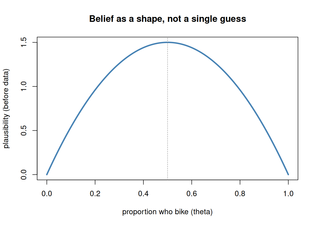
Suppose the unknown is the true proportion of students who bike to campus — a number \(\theta\) somewhere between 0 and 1. Before you collect anything, you might already believe that almost nobody (a proportion near 0) is unlikely, that almost everybody (near 1) is unlikely, and that something in the broad middle is more believable. That belief is itself a shape over the interval from 0 to 1: low at the edges, fuller in the middle. It is not a guess of one value; it is a statement about all the values at once.
This is the central reframing of the whole course. A “point” — a single number like 0.35 — throws away the part you most need: how sure are you? A shape keeps it. Two people can both say “my best guess is 0.35” and mean wildly different things: one is nearly certain, the other is barely leaning. Their shapes differ even though their points agree. Bayesian statistics insists you keep the shape.
set.seed(1)theta <-seq(0, 1, length.out =400)prior <-dbeta(theta, 2, 2) # a mild "middle is more plausible" beliefplot(theta, prior, type ="l", lwd =3, col ="steelblue",xlab ="proportion who bike (theta)", ylab ="plausibility (before data)",main ="Belief as a shape, not a single guess")abline(v =0.5, lty =3, col ="gray50")
Figure 1: A mild prior belief about the proportion of students who bike to campus: most plausibility sits in the broad middle, with values near 0 and near 1 treated as less believable before any data.
Notice we are not yet calling this a Beta distribution or doing any arithmetic with it — we will, in Week 3. For now the picture is the point: uncertainty has a shape.
The three-part motion: prior, evidence, updated belief
Bayesian reasoning is one repeated motion. Strip away every formula and it is just three words: prior, evidence, update.
You start with a prior — your current shape of plausibility.
New evidence arrives — data that fit some values better than others.
You update — you reshape your belief to respect both the prior and the evidence.
The key idea, which the rest of the course makes mathematically exact, is that the update is a compromise, not a replacement. A small amount of data nudges your shape a little; a large amount of data dominates it and the prior fades into the background. This is not a bug to be apologized for — it is exactly how a careful reasoner behaves. You do not throw out everything you knew because of one observation, and you do not cling to your starting belief in the face of a mountain of evidence.
Two features of this motion are worth naming now, because they recur all term:
Direction. Evidence pulls your belief toward the values that explain the data well. If you see a lot of bikers, plausibility shifts upward (toward larger proportions). If you see almost none, it shifts down.
Confidence. Evidence usually narrows the shape — it makes you more sure, so the hump gets taller and tighter. More data, more narrowing.
Watch direction and narrowing together as you read every example below. They are the signature of Bayesian updating.
Evidence does not erase the prior — it bends it
A common first reaction is to think the data simply “tells you the answer,” so why bother with a prior at all? Hold that thought; we will turn it into our misconception of the week. The honest picture is that both inputs matter, and how much each matters depends on how much data you have.
With little data, your prior carries real weight: the update is a gentle bend. With lots of data, the prior’s influence shrinks and the data lead: the update is a hard pull. This is reassuring in both directions. It means that if two careful analysts start with different reasonable priors, enough shared evidence will bring their conclusions close together — the data eventually win. And it means that when data are scarce, being explicit about your starting assumptions is not cheating; it is the only honest way to reason.
Worked examples
We work the running case first, then transfer the identical motion to a new context.
Worked example — bike-to-campus plausibility, before and after
Here is the running case we return to all term. We want the true proportion \(\theta\) of students who bike to campus.
Before data (the prior). We do not start blank. From walking around campus, we doubt the proportion is near 0 (some people clearly bike) and doubt it is near 1 (most clearly do not), and we lean toward “a modest minority.” A reasonable, mild way to say this is the hump-shaped belief in Figure 1 — concretely, a Beta(2, 2) prior. The “2, 2” just means a gentle preference for the middle with no strong commitment; its average is right at 0.5. We are deliberately not overconfident, because we genuinely do not know much yet.
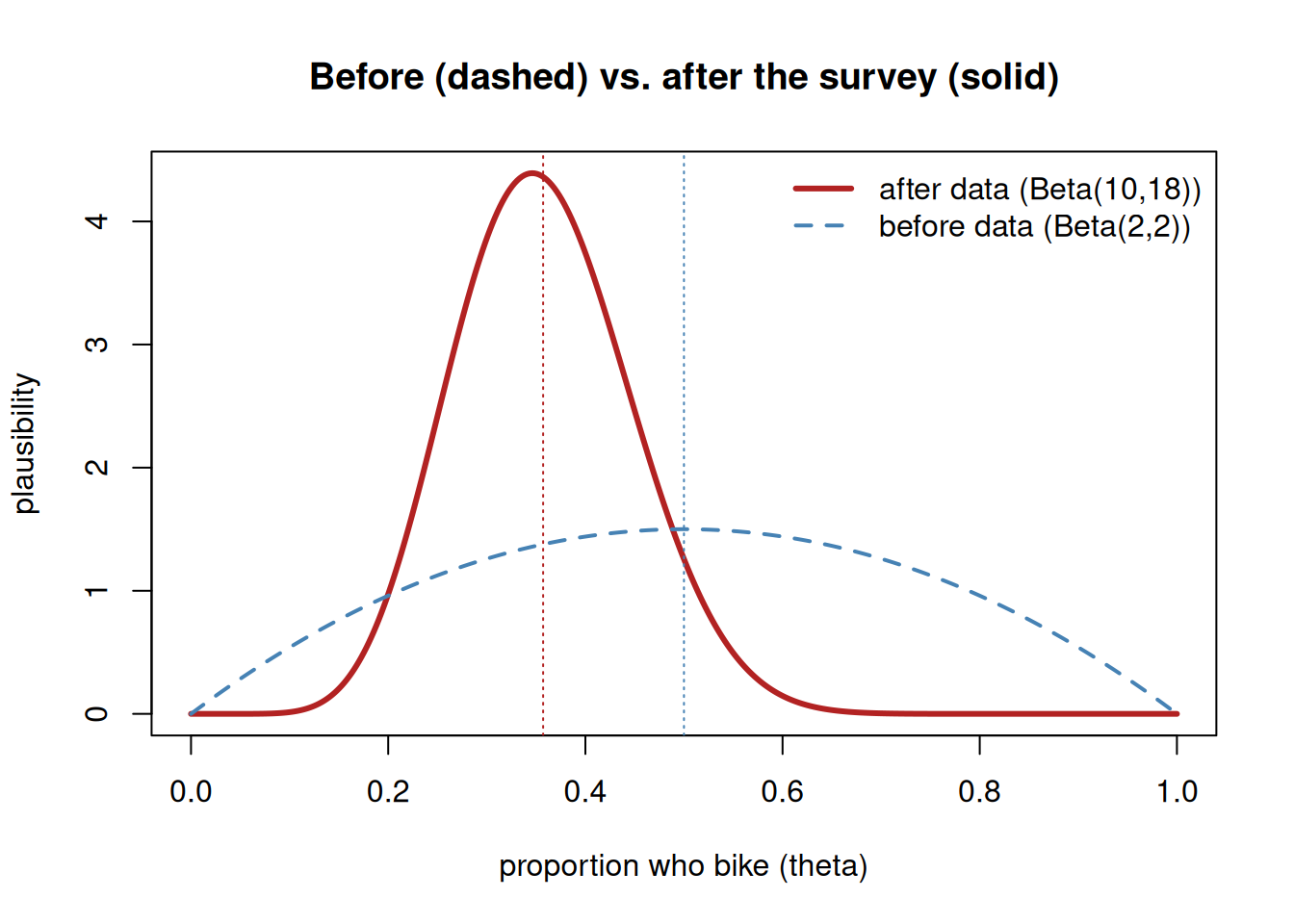
The evidence. We run a small synthetic survey: of 24 students asked, 8 say they bike. Taken alone, that raw fraction is \(8/24 \approx 0.33\).
After data (the update). Combining the mild prior with these 8-of-24 data gives an updated belief that — when we make it precise in Week 3 — is a Beta(10, 18) shape, with an average of \(10/(10+18) = 10/28 \approx 0.357\). You do not need to verify that arithmetic yet; the point is the story it tells:
The shape moved off the symmetric prior toward the data: its center slid from 0.5 down to about 0.36, because the survey suggested bikers are a minority.
The shape narrowed: seeing 24 responses made us more sure than we were with no data at all, so the updated hump is tighter than the prior hump.
The result is a compromise. The updated center, about 0.357, sits between the prior’s 0.5 and the raw data’s 0.33 — pulled most of the way to the data, but not all the way, because the prior still counts a little with only 24 responses.
set.seed(2)theta <-seq(0, 1, length.out =400)prior <-dbeta(theta, 2, 2) # before dataposterior <-dbeta(theta, 10, 18) # after 8 of 24: Beta(2+8, 2+16)plot(theta, posterior, type ="l", lwd =3, col ="firebrick",xlab ="proportion who bike (theta)", ylab ="plausibility",main ="Before (dashed) vs. after the survey (solid)")lines(theta, prior, lwd =2, lty =2, col ="steelblue")abline(v =10/28, lty =3, col ="firebrick") # updated center ~0.357abline(v =0.5, lty =3, col ="steelblue") # prior center 0.5legend("topright", c("after data (Beta(10,18))", "before data (Beta(2,2))"),col =c("firebrick", "steelblue"), lwd =c(3, 2), lty =c(1, 2), bty ="n")
Figure 2: The same belief before and after evidence. The dashed prior (mild, centered at 0.5) becomes the solid updated belief after a survey of 8 bikers out of 24: the shape shifts toward the data (lower) and gets tighter (more certain).
Everything in this picture is qualitative for now — moved and narrowed — and that is enough this week. Week 3 supplies the rule that produces Beta(10, 18) exactly.
Worked example — transfer: is this coin fair?
Now the same motion in a new context, to show it is general. The unknown is a coin’s true probability \(\theta\) of landing heads. “Fair” means \(\theta = 0.5\).
Before data (the prior). Most coins you meet are close to fair, so a sensible starting shape is one that is plausible across the middle but does not bet the house on exactly 0.5 — again a mild hump centered at 0.5. You are open to the coin being a little biased, just not wildly so.
The evidence, in stages. Suppose you flip it and get heads, heads, heads — three heads in a row.
After 1 flip (a head), your belief barely budges: one flip is almost no evidence. The shape leans a hair toward higher \(\theta\) but stays wide.
After 3 flips (all heads), it leans more noticeably toward higher \(\theta\), but you are still not ready to declare the coin loaded — three heads happens with a fair coin about one time in eight.
After 30 flips with, say, 27 heads, the shape pulls hard toward high \(\theta\) and tightens a lot. Now “fair” looks genuinely implausible.
The lesson transfers cleanly from the bike case: direction (each head pushes plausibility toward higher \(\theta\)) and narrowing (more flips means a tighter shape, more certainty). Same motion, different story. A coin is not a campus survey, but thinking under uncertainty treats them identically: start with a shape, let evidence bend it, read off the updated shape.
Notice too how the amount of evidence governs the size of the bend — three flips barely move you, thirty flips move you a lot. That is the “little data nudges, lots of data dominates” idea made concrete.
A common mistake
The trap: “a prior is just bias — real analysis should let the data speak for itself.”
This sounds principled, but it misunderstands what a prior is and smuggles in a hidden assumption. Two corrections:
First, there is no view from nowhere. Choosing to ignore prior knowledge is itself a choice — it quietly assumes every value is equally plausible to start, which is often a worse assumption than your honest knowledge. If you genuinely know a coin is probably close to fair, pretending you do not is not neutrality; it is discarding information.
Second, a good prior is disciplined, not arbitrary. It is meant to encode defensible background knowledge — physical limits, past studies, plain common sense — and you are expected to state it openly so others can question it. “Bias” hides its assumptions; a Bayesian prior publishes them. That is the opposite of bias.
How to catch yourself: when you feel the urge to say “just let the data speak,” ask two questions. What am I assuming if I use no prior at all? (Usually: that all values are equally believable, which is rarely true.) And would I be comfortable defending my prior out loud? If yes, it is reasoning, not bias. We will also see, in the prior-sensitivity work of Week 5, how to check whether a prior is doing too much — the honest answer to “is my prior reasonable?” is to test it, not to pretend it is not there.
Interpretation guidance
What does the bike result actually mean, and what does it not mean?
It means: after a small survey, our best single summary of the proportion who bike is about 0.357, but — crucially — we are still genuinely uncertain, and the shape (still fairly wide) is the honest report. A responsible statement is: “our updated best guess is roughly a third, and plausible values still spread on either side; with only 24 responses we are not pinning this down tightly.” We will learn in Week 4 to attach a credible interval to that point — a range we can honestly say the proportion plausibly lies in — and from the very first week the rule is: never report a point estimate alone. A lone “0.357” hides exactly the uncertainty this course exists to respect.
It does not mean: the true proportion is 0.357 — that is just the center of a spread, not a fact. It does not mean the survey “proved” anything; 24 responses are a small nudge, and more data could still move the picture. And it does not mean the prior was “wrong” because the center moved off 0.5 — the prior was a reasonable starting point that the evidence then revised, which is the system working as designed.
A note on language, because it matters all term: we will say a posterior gives a credible interval (a direct probability statement about where the unknown plausibly is), and we will be careful not to call it a confidence interval — those come from classical statistics and mean something different. We make that contrast precise in Week 4; for now, just register that the words are not interchangeable.
Practice (ungraded)
Use these to check your understanding. They have no posted answers — work them in your notes or bring them to discussion.
In your own words, why is “describe the unknown with a shape” more honest than “give one best-guess number”? Give one situation where the difference would actually change a decision.
For the bike case, the prior center was 0.5, the raw data fraction was about 0.33, and the updated center was about 0.357. Explain in words why the updated center landed between the other two, and closer to the data.
Suppose the survey had reached 240 students and found 80 bikers (the same fraction, 1/3, but ten times the data). Without computing anything, say what would happen to the position and the width of the updated shape compared with the 8-of-24 result, and why.
Restate the “a prior is just bias” objection as strongly as you can, then give your best one-sentence rebuttal.
Take a brand-new context — say, the probability that a particular bus is late on a given morning — and walk it through the three-part motion: a reasonable prior, what evidence you would gather, and how seeing that evidence would move and narrow your belief.
Reading guide
This week maps to Bayes Rules! Chapter 1 — The Big (Bayesian) Picture.
Read Chapter 1 for its overall arc: that Bayesian analysis is a way of updating belief in light of evidence, and that the same logic applies whether the unknown is a proportion, a rate, or anything else. As you read, line the chapter’s framing up with this note’s three-part motion (prior -> evidence -> updated belief) — they are the same idea in different words. Where the chapter contrasts the Bayesian stance with the classical one, connect it to our uncertainty is a shape, not a point section and to the credible-vs-confidence language flagged above; the Bayes-vs-classical cheat sheet summarizes that contrast. You can read Chapter 1 comfortably before attempting the practice prompts; no formulas are required yet — that is exactly the chapter’s (and this week’s) intent.
Bayes Rules! is used here as our open spine (CC BY-NC-SA 4.0); the framing and examples on this page are the course’s own, written to support that reading rather than reproduce it.
Public vs. graded
This is a public, ungraded note. The practice prompts above are for your own learning; no answer keys are posted here, and nothing on this page carries points or a due date. For anything graded — quizzes, the exit ticket, due dates, and how your work is scored — the LMS (Blackboard) is authoritative. If a graded prompt and this page ever seem to disagree, follow the LMS.
Looking ahead
Next week we make the update mechanical for the first time: Week 2 — Discrete Bayes & diagnostic reasoning takes the prior -> evidence -> updated motion and runs it through a small table of possibilities, using the classic medical-test puzzle to show how easily intuition goes wrong and how the bookkeeping sets it right.
See also
Labs overview — the reproducible computation strand (this week has no lab; the first is Lab 4).