set.seed(35103)

mu_a   <- 50     # the specific alternative being evaluated
se     <- 2.5    # SE(x-bar), n = 36, known sigma = 15
x_crit <- 49.11  # rejection-region critical value derived above (alpha = 0.05, one-sided)

n_sim <- 100000
simulated_xbars <- rnorm(n_sim, mean = mu_a, sd = se)

simulated_power <- mean(simulated_xbars > x_crit)
simulated_power # compare to the closed-form Power ~ 0.639Week 9 — Error rates, power, and decisions
Type I and Type II error, statistical power, and the trade-offs behind a testing decision
Mathematical goal
Last week’s note built a hypothesis test and showed how to read a p-value correctly. This week’s mathematical goal is to look underneath that test at the two ways it can go wrong, and to derive, from first principles, how likely each kind of error is. Concretely: given a significance level \(\alpha\), a null value \(\mu_0\), a sample size \(n\), and a standard error \(SE(\bar{x})\), derive the rejection-region critical value that a test statistic must clear to reject \(H_0\); then, given a specific alternative value \(\mu_a\), derive the test’s power — the probability the test correctly rejects \(H_0\) when that specific alternative is true. The derivation is symbolic first, then carried through the MAC Study’s own numbers.
The week question
You have already learned to ask “is this p-value small enough to reject \(H_0\)?” This week asks a different, earlier question: before you ever collect the data, how good is this test going to be at its job? A test’s job is to distinguish two states of the world — \(H_0\) true or a specific alternative \(H_a\) true — using a finite, noisy sample. No test can do this perfectly. The week’s question is how to quantify the two ways it fails (rejecting a true \(H_0\); failing to reject a false one) and how the choices you make in advance — the significance level \(\alpha\) and the sample size \(n\) — trade those failure rates against each other.
Notation
| Symbol | Meaning |
|---|---|
| \(H_0\) | Null hypothesis — the claim tested, here \(H_0: \mu = 45\) |
| \(H_a\) | Alternative hypothesis — here a specific one-sided alternative, \(H_a: \mu = 50\) |
| \(\alpha\) | Significance level — \(P(\text{reject } H_0 \mid H_0 \text{ true})\), chosen in advance |
| Type I error | Rejecting \(H_0\) when \(H_0\) is actually true; probability \(= \alpha\) |
| Type II error | Failing to reject \(H_0\) when \(H_a\) is actually true; probability \(= \beta\) |
| \(\beta\) | Type II error probability, evaluated against a specific alternative value |
| Power | \(1 - \beta\) — the probability of correctly rejecting \(H_0\) when that specific \(H_a\) is true |
| \(\bar{x}\) | Sample mean (the test statistic’s raw form here) |
| \(n\) | Sample size |
| \(\sigma\) | Population standard deviation (treated as known this week, per the course’s running convention) |
| \(SE(\bar{x})\) | Standard error of \(\bar{x}\), \(= \sigma/\sqrt{n}\) |
| \(\bar{x}_{crit}\) | The critical value of \(\bar{x}\) marking the boundary of the rejection region |
| \(z_\alpha\) | The \(z\)-value with area \(\alpha\) above it under the standard normal curve |
| \(\Phi(\cdot)\) | Standard normal cumulative distribution function |
| \(Z\) | A standard normal random variable, \(Z = (\bar{x} - \mu)/SE(\bar{x})\) under whichever \(\mu\) is assumed true |
Conceptual setup
Two populations, two ways to be wrong
A hypothesis test is a decision rule applied to data that in truth came from one of (at least) two possible worlds: the world where \(H_0\) is true, or the world where some alternative is true. The test does not know which world it is in — it only sees a sample. Because of that, there are exactly two ways the test’s decision can be wrong, and the ways depend on which world is actually the case:
- If \(H_0\) is actually true, but the sample happens to look extreme enough that the test rejects \(H_0\) anyway, that is a Type I error — a false positive. Its probability is exactly \(\alpha\), because \(\alpha\) is defined as \(P(\text{reject } H_0 \mid H_0 \text{ true})\). You do not have to derive this one; it is chosen when you set \(\alpha\).
- If \(H_a\) is actually true, but the sample happens to look ordinary enough that the test fails to reject \(H_0\), that is a Type II error — a false negative. Its probability is \(\beta = P(\text{fail to reject } H_0 \mid H_a \text{ true})\). Unlike \(\alpha\), \(\beta\) is not a number you choose directly — it falls out of \(\alpha\), \(n\), \(\sigma\), and, critically, how far the specific alternative is from the null.
Power is simply the complement of a Type II error: \(\text{Power} = 1 - \beta = P(\text{reject } H_0 \mid H_a \text{ true})\). Power answers the question “if this specific alternative is actually the truth, how often will this test notice?”
Table — the four possible outcomes of a test decision. Every test decision crosses two things that are never known to the analyst at decision time (which world is actually true) against two things the analyst does control (the decision made):
| \(H_0\) is actually true | \(H_a\) is actually true | |
|---|---|---|
| Test rejects \(H_0\) | Type I error — rate \(\alpha\) | correct decision — rate \(=\) Power \(= 1-\beta\) |
| Test fails to reject \(H_0\) | correct decision — rate \(1-\alpha\) | Type II error — rate \(\beta\) |
Read the table by column, not by row: each column is one “world,” and the two cells in that column must add to 1 (they are the only two things that can happen once you fix which world is real). The left column’s total error budget is \(\alpha\), fixed in advance; the right column’s split between Power and \(\beta\) is what the rest of this section derives.
A convention warning belongs right here, before any arithmetic: \(\beta\) and Power are only meaningful relative to a specific alternative value. There is no such thing as “the” power of a test in the abstract — only its power against \(H_a: \mu = 50\), or against \(H_a: \mu = 47\), and so on. Move the alternative closer to \(H_0\) and power drops; move it farther away and power rises. This is why the derivation below fixes a specific alternative before computing anything.
The table above is entirely abstract until the two “worlds” it names are drawn as two actual distributions, side by side.

From a decision rule to a rejection region
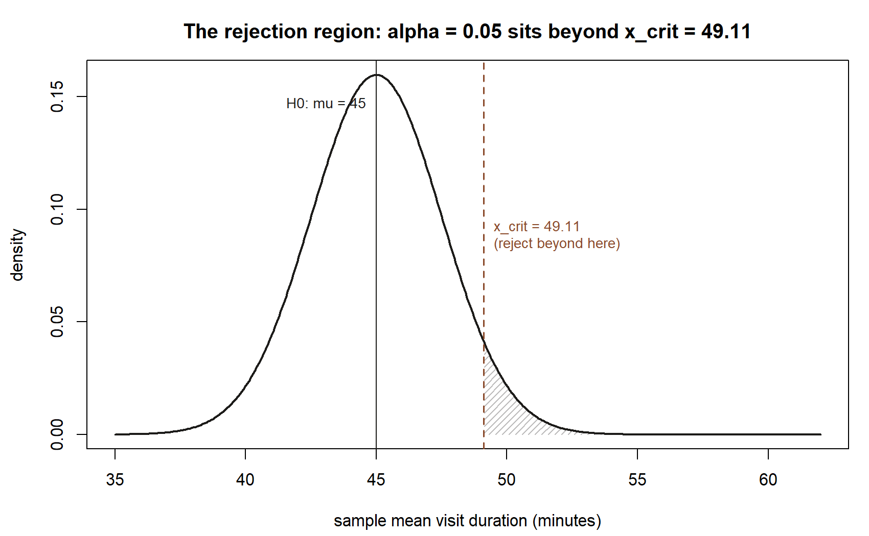
A one-sided test of \(H_0: \mu = \mu_0\) against \(H_a: \mu > \mu_0\) rejects \(H_0\) when the sample mean \(\bar{x}\) is large enough to be implausible under \(H_0\). “Large enough” has to be pinned to a precise boundary before the data are ever seen — that boundary is the critical value \(\bar{x}_{crit}\). Everything the test needs to do — control the Type I error rate, and only afterward let you compute power — flows from choosing this boundary correctly.
Deriving the critical value
Start from the definition of \(\alpha\) under \(H_0\). If \(H_0: \mu = \mu_0\) is true, then \(\bar{x}\) is approximately normal with mean \(\mu_0\) and standard error \(SE(\bar{x}) = \sigma/\sqrt{n}\) (by the sampling- distribution result from Week 2, applied under the null). The rejection region for a one-sided, upper-tailed test is \(\{\bar{x} > \bar{x}_{crit}\}\), and \(\alpha\) is defined as the probability of landing in that region when \(H_0\) is true:
\[ \alpha = P(\bar{x} > \bar{x}_{crit} \mid \mu = \mu_0) = P\!\left(Z > \frac{\bar{x}_{crit} - \mu_0}{SE(\bar{x})}\right) \]
where \(Z\) is standard normal under \(H_0\). Let \(z_\alpha\) denote the \(z\)-value with exactly \(\alpha\) of the standard normal area above it — that is, \(P(Z > z_\alpha) = \alpha\). Matching this to the expression above requires
\[ \frac{\bar{x}_{crit} - \mu_0}{SE(\bar{x})} = z_\alpha \quad\Longrightarrow\quad \bar{x}_{crit} = \mu_0 + z_\alpha \cdot SE(\bar{x}). \]
This is the rejection-region critical value: the sample mean must exceed \(\mu_0\) by at least \(z_\alpha\) standard errors before the test rejects \(H_0\). Everything about \(\alpha\) is baked into this one boundary — choosing \(\alpha\) in advance is exactly choosing how far out \(\bar{x}_{crit}\) sits.
Deriving power against a specific alternative
Now switch which world you are computing probabilities under. Power asks: if the true mean is some specific \(\mu_a \neq \mu_0\) (with \(\mu_a > \mu_0\) for this upper-tailed setup), what is the probability that \(\bar{x}\) still lands in the same rejection region \(\{\bar{x} > \bar{x}_{crit}\}\)? The rejection region itself does not move — it was fixed by \(\alpha\) under \(H_0\) — but the sampling distribution of \(\bar{x}\) now has a different center, \(\mu_a\) instead of \(\mu_0\), with the same standard error (since \(\sigma\) and \(n\) are unchanged):
\[ \text{Power} = P(\bar{x} > \bar{x}_{crit} \mid \mu = \mu_a) = P\!\left(Z > \frac{\bar{x}_{crit} - \mu_a}{SE(\bar{x})}\right) = \Phi\!\left(\frac{\mu_a - \bar{x}_{crit}}{SE(\bar{x})}\right). \]
The last step uses \(P(Z > c) = 1 - \Phi(c) = \Phi(-c)\). This single expression is the whole derivation’s payoff: power is a normal-cdf evaluation, using the same critical value derived above but re-centered on the alternative. Substituting \(\bar{x}_{crit} = \mu_0 + z_\alpha \cdot SE(\bar{x})\) gives power fully in terms of the primitives \(\alpha\), \(n\), \(\sigma\), \(\mu_0\), and \(\mu_a\):
\[ \text{Power} = \Phi\!\left(\frac{\mu_a - \mu_0}{SE(\bar{x})} - z_\alpha\right), \qquad \beta = 1 - \text{Power}. \]
Reading this closed form tells you, without any further arithmetic, what moves power: a bigger gap \(\mu_a - \mu_0\) pushes power up; a smaller \(SE(\bar{x})\) (achieved by a larger \(n\), since \(SE(\bar{x}) = \sigma/\sqrt{n}\)) pushes power up; and a larger \(z_\alpha\) (a stricter, smaller \(\alpha\)) pushes power down.
Worked example
Symbolic statement
\(H_0: \mu = 45\) versus a specific one-sided alternative \(H_a: \mu = 50\) (note: this is not a general \(H_a: \mu > 45\) — power is only defined relative to this one specific value). One-sided \(\alpha = 0.05\), so \(z_\alpha = z_{0.05} = 1.645\). Sample size \(n = 36\), known \(\sigma \approx 15\) (the course’s running known-\(\sigma\) teaching simplification), so \(SE(\bar{x}) = \sigma/\sqrt{n} = 15/6 = 2.5\).
Numeric — the MAC Study
This is the MAC Study’s visit-duration thread, continuing from Week 8’s test. There, the actual sample (\(n=36\), \(\bar{x} = 49.8\)) was tested against \(H_0: \mu = 45\) two-sided and gave \(p \approx 0.055\). This week asks a design question instead of re-testing that same sample: if the true mean visit duration really were \(\mu_a = 50\) minutes — a hypothetical value, used here purely as a specific alternative to evaluate the test against, exactly as flagged in this course’s hypothetical-vs.-sample-data convention — how good would a one-sided test at \(\alpha = 0.05\) be at detecting it, with \(n = 36\)?
Step 1 — critical value.
\[ \bar{x}_{crit} = \mu_0 + z_\alpha \cdot SE(\bar{x}) = 45 + 1.645(2.5) = 45 + 4.1125 = 49.1125 \approx \mathbf{49.11}. \]
A one-sided test at \(\alpha = 0.05\) will reject \(H_0: \mu = 45\) only if the observed sample mean exceeds \(49.11\).
Step 2 — power against \(\mu_a = 50\).
\[ \text{Power} = P(\bar{x} > 49.11 \mid \mu = 50) = P\!\left(Z > \frac{49.11 - 50}{2.5}\right) = P(Z > -0.355). \]
By symmetry of the standard normal, \(P(Z > -0.355) = \Phi(0.355)\). Looking this up (or computing it), \(\Phi(0.355) \approx \mathbf{0.639}\). So
\[ \text{Power} \approx 0.639, \qquad \beta = 1 - \text{Power} \approx \mathbf{0.361}. \]
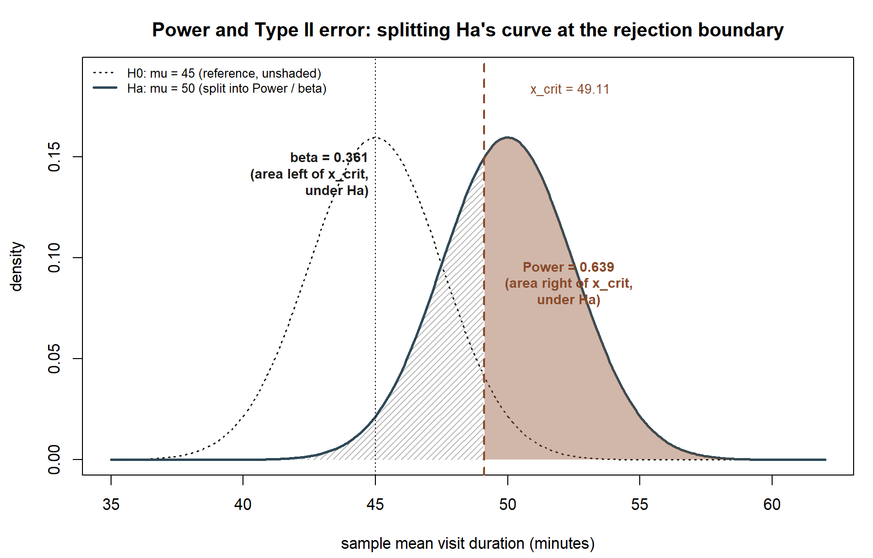
Reading the result. If the true mean visit duration were really 50 minutes, this test — one-sided, \(\alpha = 0.05\), \(n = 36\) — would correctly reject \(H_0: \mu = 45\) only about 64% of the time. About 36% of the time, it would fail to detect a real, 5-minute shift in the mean, purely due to sampling variability. This is a meaningfully high Type II error rate for a difference many researchers would care about detecting, and it is the kind of number a researcher should know before running the study, not after failing to find significance.
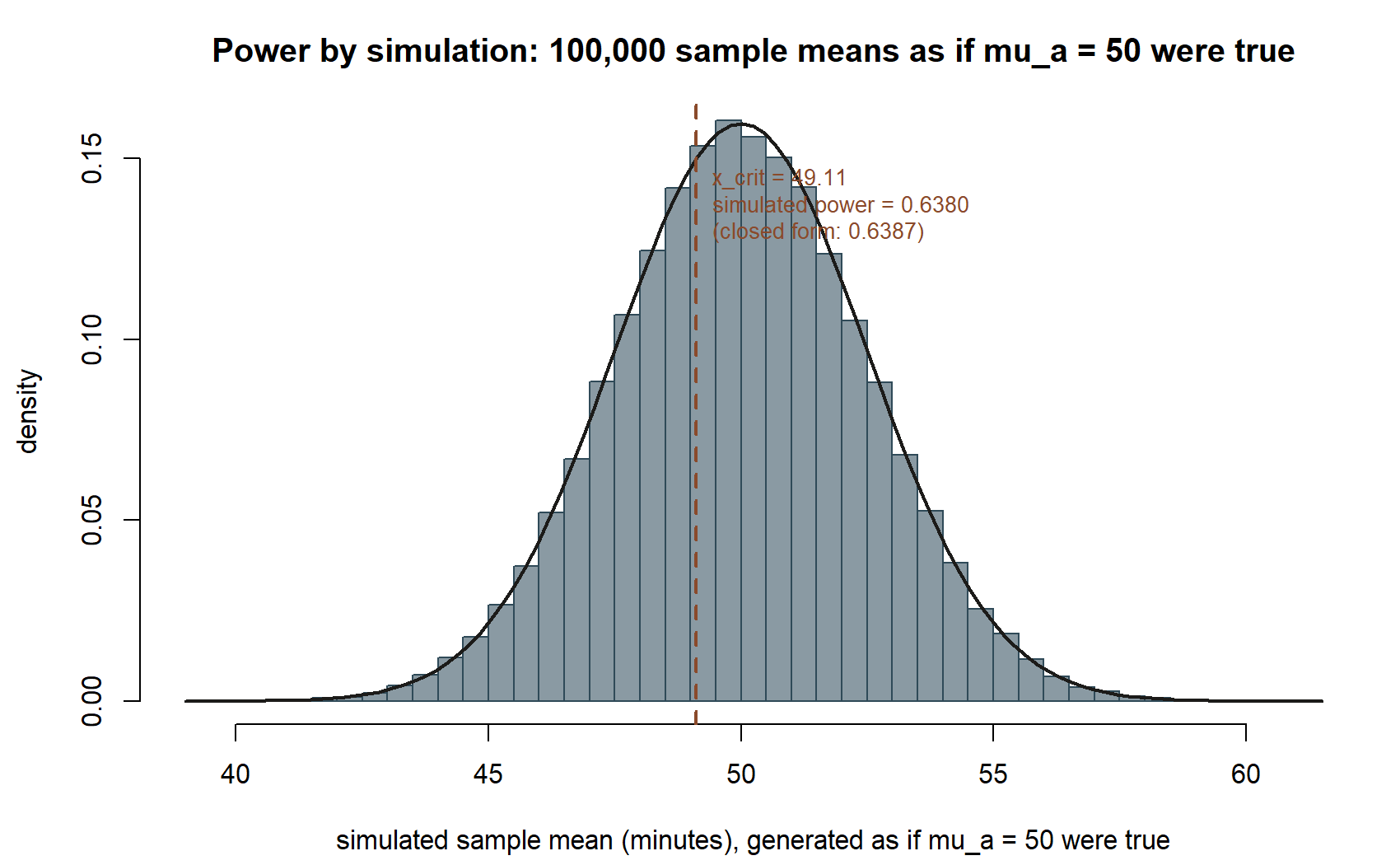
Seeing power by simulation, as a cross-check on the closed form. The derivation above computes power as a single normal-cdf evaluation. The same number can be approximated directly by simulation: repeatedly generate sample means as if the alternative \(\mu_a = 50\) were the true mean, and count how often each one clears the rejection-region critical value \(\bar{x}_{crit} = 49.11\).
What this shows (public-safe description, since this chunk is not executed here): among 100,000 simulated sample means generated as if the true mean really were \(\mu_a = 50\), the fraction exceeding the critical value \(49.11\) approximates the closed-form power of \(0.639\) — the same “reject or not” decision rule, applied repeatedly to hypothetical data from the alternative world, converges to the same number the normal-cdf derivation gives directly.
Transfer example — factory defect-rate detection (synthetic; seed set)
A quality-control team wants to know whether a new machine setting has increased a factory’s defect rate above the historical baseline. This is a fresh, synthetic context, distinct from the MAC Study, used only to show that the same derivation transfers to a different setting and a different kind of specific alternative. (In a full course build this would be developed as a proportion test rather than a mean test; here it is kept in the same mean-based form as the derivation above, applied to a hypothetical “average defects per batch” measure, so the arithmetic mirrors the MAC Study step for step and the reader can check the mechanics independently.)
Suppose historical baseline average defects per batch is \(\mu_0 = 8.0\), with known process standard deviation \(\sigma = 6.0\) (synthetic values, not from any real vendor data), and quality control samples \(n = 36\) batches under the new setting, so \(SE(\bar{x}) = 6.0/\sqrt{36} = 6.0/6 = 1.0\). Testing one-sided at \(\alpha = 0.05\) (\(z_{0.05} = 1.645\)) for an increase:
\[ \bar{x}_{crit} = 8.0 + 1.645(1.0) = 9.645. \]
Suppose the team wants to know this test’s power if the new setting actually raised the true average to \(\mu_a = 10.0\) defects per batch (synthetic hypothetical alternative):
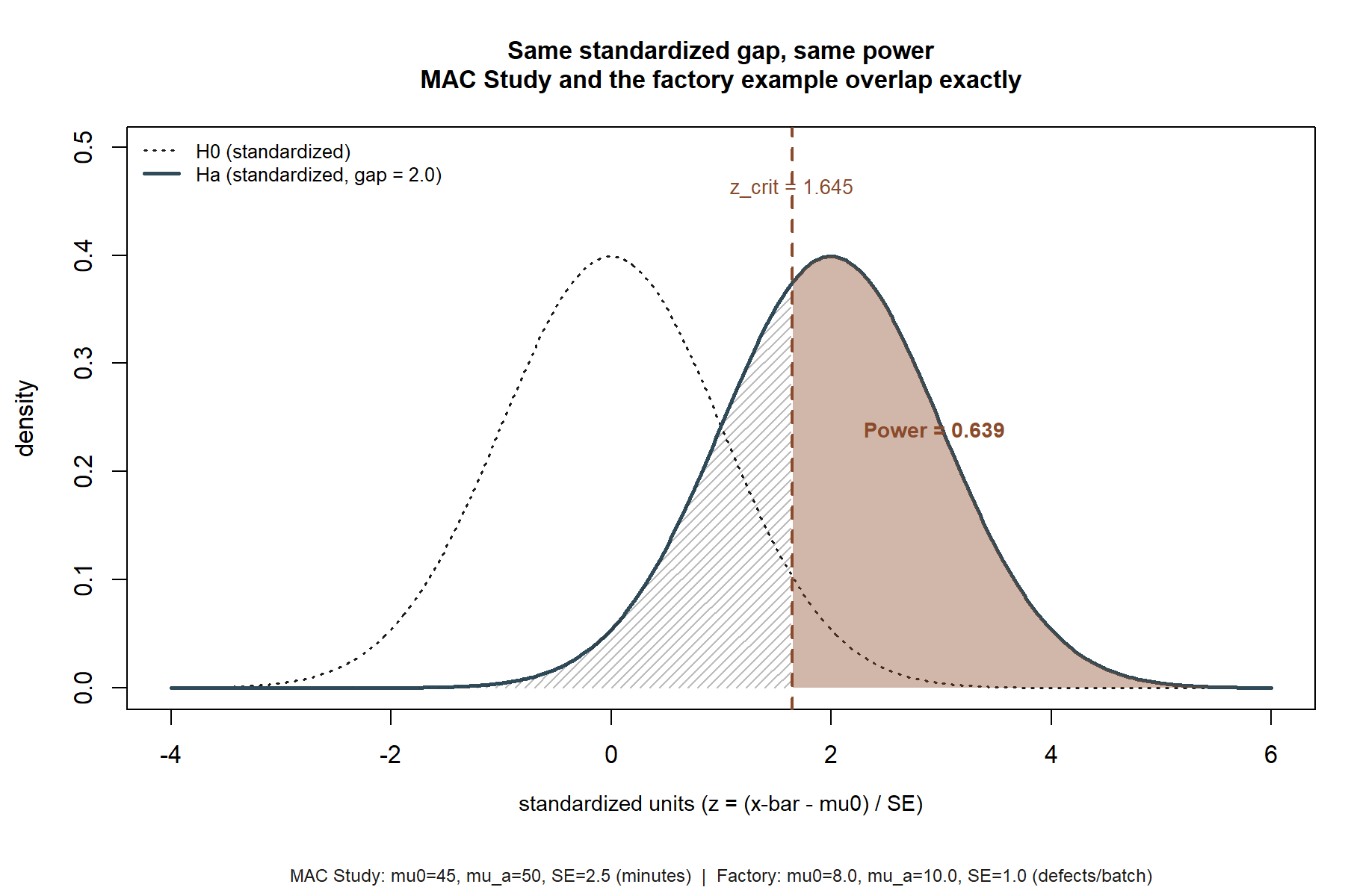
\[ \text{Power} = P(\bar{x} > 9.645 \mid \mu = 10.0) = P\!\left(Z > \frac{9.645 - 10.0}{1.0}\right) = P(Z > -0.355) = \Phi(0.355) \approx 0.639. \]
By design, this transfer example was built so the standardized distance \((\mu_a - \bar{x}_{crit})/SE(\bar{x})\) comes out to the same \(-0.355\) as the MAC Study case, so it lands on the identical power, \(\approx 0.639\), \(\beta \approx 0.361\) — a deliberate illustration that power depends only on the standardized gap between \(\bar{x}_{crit}\) and \(\mu_a\), not on the underlying units or context. A factory’s defect count and a MAC visit duration have nothing in common substantively, but once the problem is expressed in standard-error units the same normal-curve calculation applies.
The trade-offs
Three levers appear in the closed-form power expression above, and each is worth naming explicitly, because this is exactly the kind of design decision a real study makes before collecting data.
- Raising \(\alpha\) raises power, but raises the false-positive rate. A larger \(\alpha\) means a smaller \(z_\alpha\), which pulls \(\bar{x}_{crit}\) closer to \(\mu_0\) — easier to cross, hence higher power against any fixed alternative. But \(\alpha\) is the Type I error rate, so this “buys” power directly at the cost of more false rejections of a true \(H_0\). There is no way to lower \(\beta\) by raising \(\alpha\) without also raising the Type I error rate — the two errors trade off directly at a fixed \(n\).
- Raising \(n\) raises power at a fixed \(\alpha\), without that trade-off. A larger \(n\) shrinks \(SE(\bar{x}) = \sigma/\sqrt{n}\), which pulls \(\bar{x}_{crit}\) closer to \(\mu_0\) (in standard-error terms the boundary is unchanged at \(z_\alpha\), but in raw units it tightens) while simultaneously making the sampling distribution under \(\mu_a\) narrower and better separated from \(\mu_0\). This is the reason a well-designed study prefers to solve low power by collecting more data rather than by loosening \(\alpha\) — sample size is the lever that improves both error rates’ balance rather than swapping one for the other.
- Moving the alternative farther from the null raises power “for free,” but you do not get to choose the true alternative. A test built to detect \(\mu_a = 55\) (farther from \(\mu_0 = 45\)) would have higher power than the \(\mu_a = 50\) case above, at the same \(\alpha\) and \(n\) — but this is not a design choice; it simply reflects that bigger real effects are easier to detect. A power calculation is only useful once you commit to a specific alternative that reflects the smallest effect size you would actually care about missing.
A convention warning
Two convention-risk points from the course’s shared notation ledger apply directly here, and a third is specific to this week. First, \(\alpha\) and \(\beta\) are not symmetric partners you can shrink together at a fixed \(n\) — shrinking one (at fixed \(n\)) grows the other; only more data lets both improve together. Second, power and \(\beta\) are always relative to one specific alternative value, never a property of the test “in general” — a test has high power against \(\mu_a = 60\) and low power against \(\mu_a = 46\) simultaneously; asking “what is this test’s power?” without naming \(\mu_a\) is an incomplete question. Third, and specific to this derivation: the alternative value \(\mu_a = 50\) used above is a hypothetical value, used only as a stipulated truth so the power calculation has something concrete to evaluate against — it is never the actual, known mean visit duration, and this derivation never claims to know the sample’s true population mean. This mirrors exactly how Week 2 used a hypothetical true world to simulate a sampling distribution: a teaching device, clearly flagged, not a claim about a known population fact.
Practice (ungraded)
These are self-check prompts only — no submission, no grading, no key.
- Using the symbolic result \(\bar{x}_{crit} = \mu_0 + z_\alpha \cdot SE(\bar{x})\), recompute the critical value if \(\alpha\) were tightened to a two-sided-equivalent one-sided \(\alpha = 0.01\) (\(z_{0.01} \approx 2.326\)), keeping \(\mu_0 = 45\) and \(SE(\bar{x}) = 2.5\) from the MAC Study. Is the new critical value farther from or closer to \(\mu_0\) than \(49.11\), and does that match the direction you would expect from a stricter \(\alpha\)?
- Using the same \(\alpha = 0.05\) critical value \(\bar{x}_{crit} = 49.11\), recompute power against a different specific alternative, \(\mu_a = 52\) instead of \(50\), still with \(SE(\bar{x}) = 2.5\). Is the new power higher or lower than \(0.639\), and does that match the derivation’s prediction about moving the alternative farther from \(\mu_0\)?
- In the factory transfer example, suppose the quality-control team could only sample \(n = 9\) batches instead of \(36\), so \(SE(\bar{x}) = 6.0/\sqrt{9} = 2.0\) instead of \(1.0\). Recompute \(\bar{x}_{crit}\) (still \(\mu_0 = 8.0\), \(\alpha = 0.05\)) and then power against \(\mu_a = 10.0\). Which direction does power move compared to the \(n=36\) case, and why does that match the sample-size lever described above?
- In your own words, explain why a researcher who only reports “we failed to reject \(H_0\)” without ever having computed the test’s power against a specific, meaningful alternative has left out important information about what that non-rejection does or does not tell you.
Reading and source pointer
This week’s development of Type I/Type II error, the rejection-region critical value, and statistical power follows MIT OCW 18.05’s treatment of hypothesis testing and power (used selectively, as the course’s primary spine). These notes are the course’s own synthesis, grounded in but not copied from the source.
Public vs. graded
These notes, the examples, and the practice here are public and ungraded — study material only. No graded prompts, answer keys, rubrics, point values, or due dates appear on this site. Graded inference checkpoints, quizzes, homework, labs, the midterm, the project, and the final live in Blackboard (the LMS), which is authoritative for due dates, submissions, and grades. If this page and Blackboard ever disagree, follow Blackboard.
Looking ahead
Next week turns from a formula-based sampling distribution to a fully simulation-based one: the bootstrap builds a confidence interval by resampling the data you actually have, rather than assuming a normal sampling-distribution formula. You will see the same visit-duration sample from this week and Week 7 produce a percentile interval that lands close to, but not identical to, the normal-theory interval — a check on how much the known-\(\sigma\) simplification used here and in earlier weeks was doing for you.
See also
- Week 8 — Hypothesis tests and p-values — the test this week’s error-rate analysis is built on top of.
- Week 10 — Bootstrap inference — the next step, replacing the normal-theory sampling distribution with a resampling-based one.
- Resources — Inference formula reference — a standing collection of the course’s formulas, including this week’s critical-value and power expressions.
- Resources — Notation glossary — full definitions of \(\alpha\), \(\beta\), Power, and related symbols used throughout the course.