Lab 12 — Simulating the posterior

Recovering Beta(41, 69) by drawing from it, instead of only integrating to find it

Purpose. Week 12’s note (see Week 12 — Bayesian inference) derives, by algebra, that a Beta(a = 3, b = 7) prior on the MAC usage-rate parameter \(\pi\), updated by the full survey’s \(n = 100\), \(k = 38\) Binomial data, produces a Beta(3 + 38, 7 + 62) = Beta(41, 69) posterior, with posterior mean \(41/110 \approx 0.373\) and a normal-approximation 95% credible interval of approximately (0.283, 0.463). That derivation leans on two facts you may be willing to take on faith but have not yet watched happen: the Beta-Binomial conjugacy update itself, and the claim that a Beta(41, 69) density really does have its probability mass concentrated in that interval. This lab sets the algebra aside for a moment and recovers the same two numbers — the posterior mean and the credible interval — by simulation instead: drawing a large number of values directly from a Beta(41, 69) distribution in R and summarizing what comes out. You are not proving the conjugacy result here; you are confirming, by a completely different route, that the posterior the note derived is really shaped the way the note says it is.

The idea

Section 12’s algebra tells you that the posterior density \(\pi(\theta \mid \text{data})\) is proportional to prior times likelihood, and that for a Beta prior combined with Binomial data the proportionality works out, term by term, to another Beta density with updated parameters \(a + k\) and \(b + (n - k)\). That is an exact, closed-form statement about a whole density function — every value of \(\pi\) from 0 to 1 gets an updated “height,” and the Beta(41, 69) formula tells you exactly what that height is at every point.

Simulation takes a different, more concrete route to the same place. Instead of working with the density function, you ask R’s random-number generator to produce many individual draws — actual numbers between 0 and 1 — that behave as though they came from the Beta(41, 69) distribution. If you draw enough of them, say 50,000, and then just look at what you got — their average, their spread, the middle 95% of them — those simulated summaries should land very close to the numbers Week 12 derived by algebra: a mean near 0.373 and a middle-95% band near (0.283, 0.463). This is the same logic Lab 2 used for a sampling distribution: theory gives you an exact formula, simulation gives you a large finite pile of numbers that should look like the formula, and comparing the two is a check that both routes agree.

There is a second, smaller idea folded into this lab as well: the route by which you get simulated draws from the posterior. Because Beta and Binomial are conjugate, the posterior is itself a named Beta distribution — Beta(41, 69) — and R’s built-in rbeta() function can draw directly from any Beta distribution you specify, given its two parameters. So the most direct way to simulate this posterior is simply rbeta(50000, 3 + 38, 7 + 62): hand rbeta() the updated parameters \(a + k = 41\) and \(b + n - k = 69\), and it draws straight from the posterior with no extra machinery. (A slower, more manual alternative — drawing candidate \(\pi\) values from the Beta(3, 7) prior and using an accept/reject rule weighted by the Binomial likelihood at each candidate — would also work in principle, and is mentioned in Step 1 below for context, but this lab uses the direct rbeta() route throughout, because it is exact, fast, and is exactly what the conjugacy result in Week 12 licenses you to do.) The whole point of conjugacy, in fact, is that it tells you which named distribution to draw from directly, so you never need the slower accept/reject machinery at all once you know the posterior family.

Goal

By the end of this lab you should be able to:

• Explain, in one or two sentences, why Beta-Binomial conjugacy lets you draw directly from the posterior using rbeta() with updated parameters, rather than needing a more general accept/reject simulation.
• Draw a large number of simulated values from the Beta(41, 69) posterior using base R’s rbeta().
• Summarize those simulated draws with mean() and quantile(), and compare the simulated summaries to the Week 12 note’s algebraic posterior mean (\(\approx 0.373\)) and normal-approximation credible interval (\(\approx (0.283, 0.463)\)).
• Compare a simulation-based credible interval, built directly from the empirical quantiles of the simulated draws, to the note’s normal-approximation interval, and describe in words why the two are close but not identical.

Setup

You will need base R only — no packages beyond what ships with R. As in every simulation chunk this course uses, set your seed before drawing any random numbers, so your results match the ones described here when you run this yourself later (remember: in this build the chunks are shown, not executed).

set.seed(35103)

Recall the four numbers that anchor this whole lab, all derived algebraically in the Week 12 note and never re-derived differently here:

• Prior: Beta(a = 3, b = 7) — prior mean 3/10 = 0.30, representing the MAC director’s belief about the usage rate \(\pi\) before this term’s survey.
• Data: the full survey, n = 100, k = 38 students used the MAC at least once this week.
• Posterior (by Beta-Binomial conjugacy): Beta(3 + 38, 7 + 62) = Beta(41, 69).
• Target numbers to recover by simulation: posterior mean \(\approx 0.373\); normal-approximation 95% credible interval \(\approx (0.283, 0.463)\).

Steps

Step 1 — Draw a large number of samples directly from the Beta(41, 69) posterior

The most direct way to simulate the posterior is to hand rbeta() the updated Beta parameters straight from the conjugacy result: \(a + k = 3 + 38 = 41\) and \(b + (n - k) = 7 + 62 = 69\). Writing the arithmetic out inside the call, rather than typing 41 and 69 directly, keeps the connection to the prior and the data visible in the code itself.

set.seed(35103)

a_prior <- 3
b_prior <- 7
n       <- 100
k       <- 38

B <- 50000   # number of simulated posterior draws

post_draws <- rbeta(B, a_prior + k, b_prior + (n - k))

length(post_draws)   # should be 50000
head(post_draws)      # first few simulated posterior draws

This chunk is shown but not executed on this page (eval: false) — running it yourself is the point. The figure below was produced by running exactly this chunk’s code separately (same seed 35103, same rbeta(50000, 41, 69) call), plotted as a bare histogram before Step 4 compares it to the exact density:

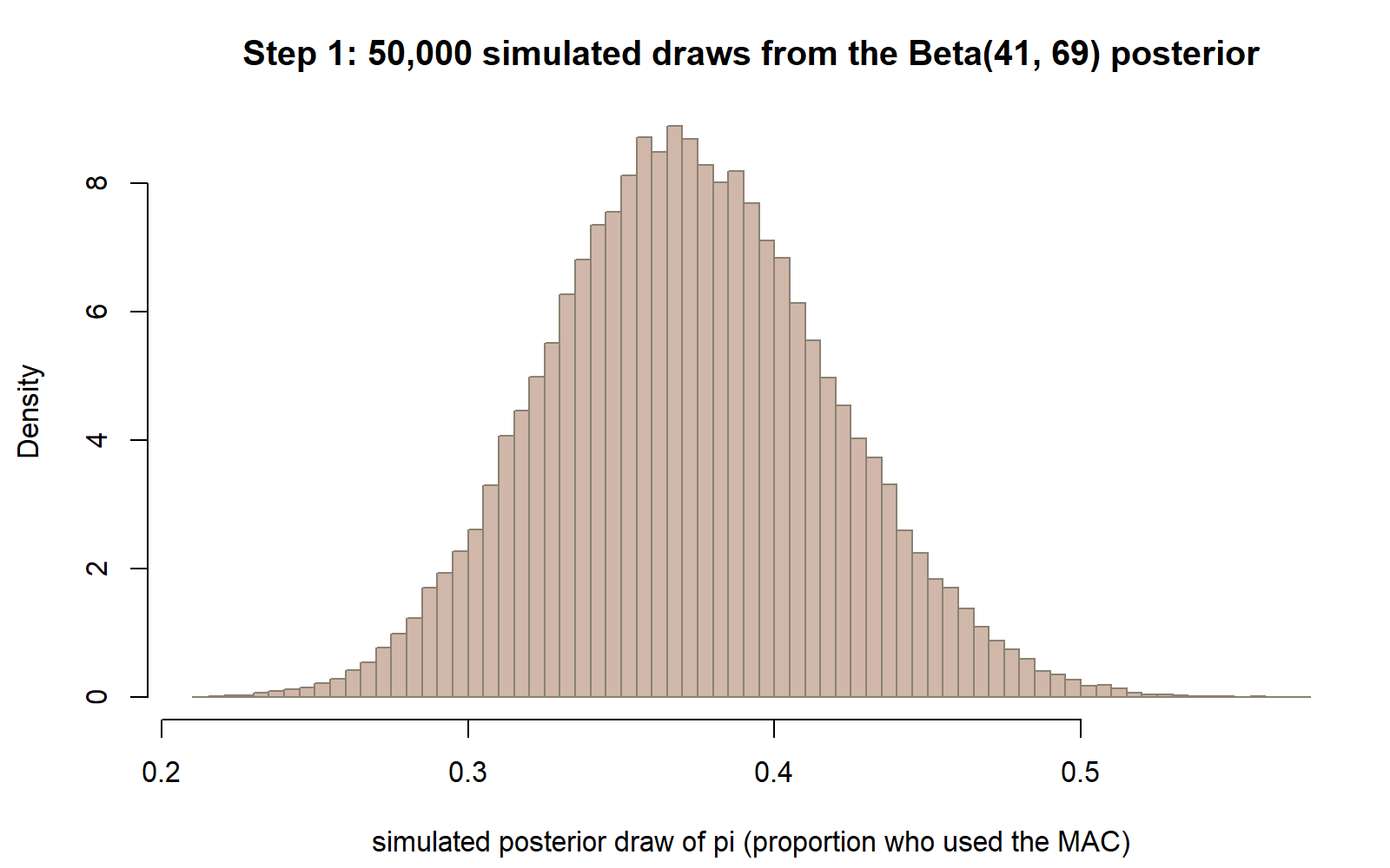
Figure 1: The simulated posterior draws, visualized (synthetic). A histogram of the 50,000 raw draws from rbeta(50000, 41, 69), before any exact density curve is overlaid — the shape you would see immediately after running Step 1.

post_draws is now a vector of 50,000 numbers, each between 0 and 1, each one an independent simulated draw from the Beta(41, 69) posterior. (A slower alternative worth knowing about, though not used further in this lab, would be an accept/reject scheme: draw a large number of candidate \(\pi\) values from the Beta(3, 7) prior with rbeta(B, a_prior, b_prior), then keep each candidate only with probability proportional to the Binomial likelihood \(\pi^{k}(1-\pi)^{n-k}\) evaluated at that candidate, discarding the rest. That scheme would, in principle, also produce draws that look like the Beta(41, 69) posterior, but it wastes most of its draws by rejection and needs a likelihood evaluation at every candidate. Conjugacy is precisely what lets this lab skip all of that and draw from the posterior directly and exactly with a single rbeta() call.)

Step 2 — Recover the posterior mean from the simulated draws

With 50,000 simulated posterior draws in hand, the posterior mean is nothing more than the plain average of those draws.

set.seed(35103)

mean(post_draws)   # expect a number close to 0.373

Compare this simulated mean to the Week 12 note’s algebraic posterior mean, \(41/110 \approx 0.373\). Because B = 50000 is large but finite, mean(post_draws) will not land on exactly 0.373 — expect small simulation noise, typically a number such as 0.372-something or 0.373-something, changing slightly if you rerun with a different seed or a different B. The point of the exercise is that the simulated mean lands close to 0.373, not that it matches to every decimal place.

This chunk is shown but not executed on this page. The figure below extends this chunk’s post_draws object with a plotting call not written on the page — tracking the cumulative mean as draws accumulate, produced by running exactly this chunk’s code separately (same seed, same B = 50000), so you can watch it settle down toward 0.373 rather than only reading off the final number:

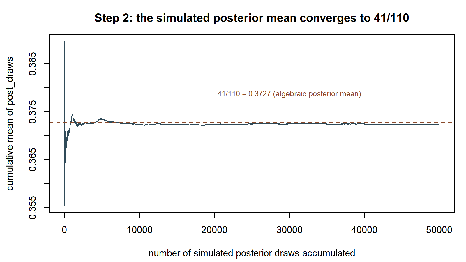
Figure 2: The simulated posterior mean converging (synthetic). As the number of accumulated draws grows from 1 to 50,000, the running mean of post_draws settles near the algebraic posterior mean \(41/110 \approx 0.3727\) — this settling-down is what “draw enough of them” is buying.

Step 3 — Recover the credible interval with quantile()

The Week 12 note reports a normal-approximation 95% credible interval, built from the posterior mean and SD plugged into \(\hat\theta \pm 1.96 \times SD\). The simulated draws let you build a credible interval a different way, with no normal approximation at all: just read off the middle 95% of the simulated draws directly, using base R’s quantile() at the 2.5th and 97.5th percentiles.

set.seed(35103)

sd(post_draws)   # expect a number close to 0.0459, the posterior SD

ci_simulated <- quantile(post_draws, probs = c(0.025, 0.975))
ci_simulated   # expect bounds close to (0.283, 0.463)

quantile(post_draws, probs = c(0.025, 0.975)) returns two numbers: the value below which 2.5% of the simulated draws fall, and the value below which 97.5% fall. The interval between them contains the middle 95% of the simulated posterior draws — a simulation-based credible interval, built directly from the shape of the simulated distribution, with no assumption that the posterior looks Normal. Compare it to the note’s normal-approximation interval, \(0.373 \pm 1.96(0.0459) \approx (0.283, 0.463)\): the two should be close, because Beta(41, 69), with both parameters well above 1 and reasonably large, is itself fairly close to Normal-shaped already — but they need not match digit for digit, since one is an exact simulated-quantile statement about a slightly-skewed Beta shape and the other is a Normal approximation to that same shape.

This chunk is shown but not executed on this page. The figure below extends this chunk’s ci_simulated object with a comparison plot not written on the page, produced by running exactly this chunk’s code separately (same seed, same post_draws):

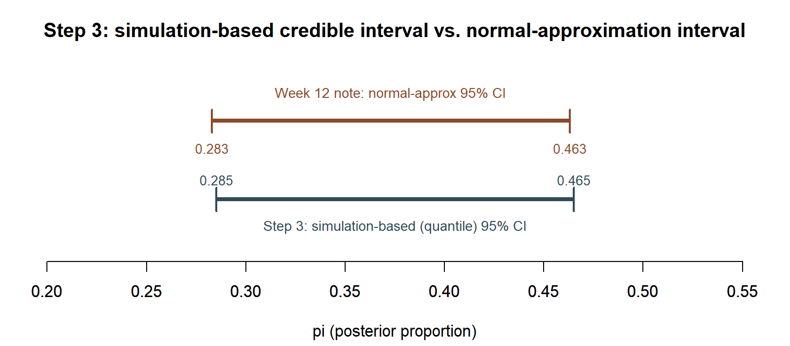
Figure 3: Simulation-based CI vs. normal-approximation CI (synthetic). For this particular run, ci_simulated = (0.285, 0.465) — close to, but not identical to, the Week 12 note’s normal-approximation interval (0.283, 0.463); both are reported here rather than treating one as simply replacing the other.

Step 4 — Visualize the simulated posterior against the Beta(41, 69) density

Finally, plot a histogram of the simulated posterior draws and overlay the exact Beta(41, 69) density curve using base R’s dbeta() and curve(), so you can see directly how closely the simulated draws track the known closed-form posterior.

set.seed(35103)

hist(post_draws,
     breaks = 60,
     freq   = FALSE,
     main   = "Simulated vs. exact Beta(41, 69) posterior",
     xlab   = "simulated posterior draw of pi")

curve(dbeta(x, a_prior + k, b_prior + (n - k)),
      add = TRUE,
      lwd = 2)

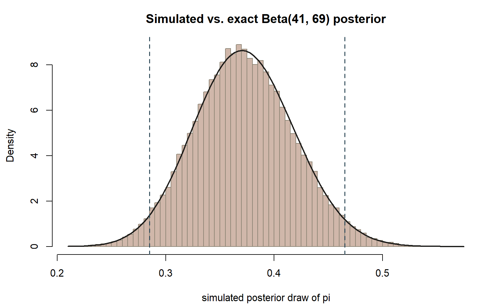
abline(v = ci_simulated, lty = 2)

If the simulation and the exact Beta(41, 69) density agree, the smooth curve should sit almost exactly on top of the histogram’s bars, peaking somewhere close to \(\pi \approx 0.373\) and tapering off toward 0 and 1. The two dashed vertical lines mark the simulation-based 95% credible interval from Step 3, and should bracket almost all of the histogram’s central mass.

This chunk is shown but not executed on this page (eval: false) — running it yourself is the point. The figure below was produced by running exactly this chunk’s hist()/curve()/abline() code separately (same seed, same post_draws and ci_simulated), so you can check your prediction against a real result:

Figure 4: Simulated draws vs. the exact Beta(41, 69) posterior (synthetic). A histogram of the 50,000 simulated posterior draws with the exact Beta(41, 69) density curve overlaid, and the Step 3 simulation-based 95% credible interval marked by dashed lines. The curve tracks the histogram’s bars closely across the whole range.

Verify

Before you consider this lab complete, check all of the following against your own output:

• length(post_draws) equals 50000 — one simulated draw per requested draw, no more and no fewer.
• Every value in post_draws is strictly between 0 and 1 — a proportion can never fall outside that range, and rbeta() guarantees this by construction.
• mean(post_draws) is close to 0.373, the Week 12 note’s algebraic posterior mean \(41/110\), not close to 0.30 (that would be the prior mean, before the survey data updated it) and not close to 0.38 (that would be the raw sample proportion \(\hat{p} = k/n\), before the prior was folded in at all).
• sd(post_draws) is close to 0.0459, the Week 12 note’s algebraic posterior SD.
• quantile(post_draws, probs = c(0.025, 0.975)) gives bounds close to (0.283, 0.463), the note’s normal-approximation credible interval — close, but not necessarily identical to the last decimal, since a simulated-quantile interval and a normal-approximation interval are two different (if closely agreeing) ways of summarizing the same posterior shape.
• The histogram from Step 4 looks unimodal, roughly bell-shaped, and centered near \(\pi \approx 0.373\), and the overlaid Beta(41, 69) curve sits close to the histogram’s bars across the whole range.
• If you rerun the whole script from the very top with set.seed(35103) restored at each chunk, you get the same post_draws values and the same summary numbers every time.

As a second, unrelated context for the same idea (synthetic; seed 35103), imagine a quality-control team with a Beta(a = 5, b = 20) prior belief about the defect rate on a production line, updated by a fresh inspection batch of n = 50 items with k = 6 defective. Beta-Binomial conjugacy gives a posterior of Beta(5 + 6, 20 + 44) = Beta(11, 64), with algebraic posterior mean \(11/75 \approx 0.1467\). Running the same four-step recipe above — rbeta(50000, 11, 64), then mean() and quantile(., c(0.025, 0.975)) on the simulated draws — would be expected to recover a simulated mean close to 0.1467 and a simulated 95% interval close to the normal-approximation band \(0.1467 \pm 1.96 \times SD\), where \(SD = \sqrt{(11 \times 64) / (75^2 \times 76)} \approx 0.0408\), giving an approximate band of about (0.067, 0.226). Nothing about the four steps changes between the MAC Study and the defect-rate example except the two posterior parameters fed into rbeta() — the same recipe (simulate from the named posterior, then summarize with mean() and quantile()) works for any Beta posterior, which is exactly what makes conjugacy such a convenient special case to simulate from.

AI use note

Tool	Purpose	Verification
AI coding assistant (e.g. Claude, ChatGPT, Copilot)	Drafting or troubleshooting base-R simulation code such as the rbeta() / mean() / quantile() pattern above, or explaining how quantile()’s probs argument selects percentiles	Run the AI-suggested code yourself in your own R session with set.seed(35103) set, and confirm length(post_draws) == 50000, mean(post_draws) near 0.373, and quantile(post_draws, probs = c(0.025, 0.975)) near (0.283, 0.463) before trusting any AI-assisted rewrite; never submit AI output you have not run and checked against these numbers

The graded deliverable, its rubric, and due date live in Blackboard (the LMS) — this page is study and practice only.

See also

• Week 12 — Bayesian inference — the companion note deriving the Beta-Binomial conjugacy result and the Beta(41, 69) posterior this lab simulates.
• Labs index — the full list of course labs.
• Notation glossary — definitions for \(\pi(\theta)\), \(\pi(\theta \mid \text{data})\), and Beta(a, b).