Lab 11 — Randomization tests

Building a permutation null distribution in base R for the workshop-vs-control comparison

Purpose. This lab is the hands-on companion to Week 11 — Randomization and permutation tests. The week note develops the logic of a randomization (permutation) test in words and works the normal-approximation cross-check by hand. Here, you build the actual permutation null distribution in code — by shuffling group labels thousands of times — and read off a permutation p-value that you can compare directly to the week note’s z-based answer.

The idea

A randomization test asks a very direct question: if the workshop label (“workshop” vs. “control”) had nothing to do with visit duration, and the two group labels had been assigned at random, how often would random label-shuffling alone produce a mean difference at least as extreme as the one we actually observed?

The logic has three moving parts, and it is worth holding all three in mind before you write any code:

1. Pool the data. Under the null hypothesis “the workshop has no effect on visit duration,” the 40 visit times you collected do not really belong to two different populations — they are 40 numbers that happened to get labeled “workshop” or “control.” If the labels are irrelevant to the outcome, we should be able to scramble them and lose nothing that matters.
2. Reshuffle and recompute. Randomly reassign the 40 labels (20 “workshop,” 20 “control”) to the 40 pooled values, over and over, and recompute the mean difference (workshop mean minus control mean) each time. This generates a distribution of mean differences that could arise by label-shuffling alone, with no real group effect.
3. Locate the observed difference in that distribution. If the actual observed difference (7.3 minutes) sits way out in the tail of the shuffled differences, that is evidence the labels are not interchangeable with the outcome after all — i.e., evidence against the null.

This is exactly the “simulation-based inference” framing that ModernDive centers for randomization and permutation tests: instead of trusting a normal-distribution formula for the null distribution of the mean difference, you construct that null distribution directly by resampling, using nothing but the assumption that labels don’t matter. This lab describes that framing in words and carries it out in base R (sample() for the shuffle, replicate() to repeat it many times) rather than the infer package’s specify()/hypothesize()/generate()/calculate() pipeline that ModernDive itself uses — same idea, base-R computation, per this course’s house style.

Goal

By the end of this lab you will have base-R code that:

• builds synthetic stand-in vectors for the workshop and control groups matching the week’s locked summary statistics (n, mean, SD for each group),
• pools the 40 values and repeatedly reshuffles the group labels B = 5000 times,
• recomputes the mean difference (workshop − control) on every shuffle to build up a permutation null distribution,
• reports a two-sided permutation p-value for the observed difference of 7.3 minutes, and
• compares that permutation p-value to the week note’s normal-approximation p ≈ 0.021.

Setup

You will need only base R — no packages. Everything below assumes a fresh R session.

set.seed(35103)

# Locked summary statistics from the week-11 note (do not change these):
n_workshop <- 20
mean_workshop <- 52.4
sd_workshop <- 10

n_control <- 20
mean_control <- 45.1
sd_control <- 10

observed_diff <- mean_workshop - mean_control
observed_diff

This chunk is shown but not executed on this page (eval: false) — running it yourself is the point. The figure below was produced by running exactly this chunk’s code separately (same locked summary statistics), turning the two locked group means into a picture before any resampling begins:

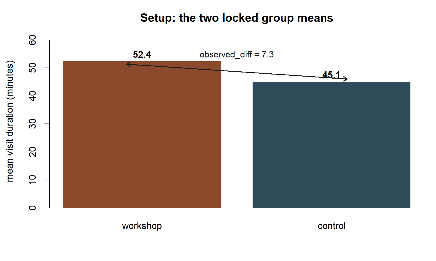
Figure 1: The two locked group means and the observed difference (synthetic). Workshop mean 52.4 minutes vs. control mean 45.1 minutes; the gap between them, observed_diff = 7.3 minutes, is the number every later step in this lab is trying to locate inside a null distribution.

observed_diff should print 7.3 (technically 7.300000000000004 or similar due to floating-point subtraction — treat it as 7.3).

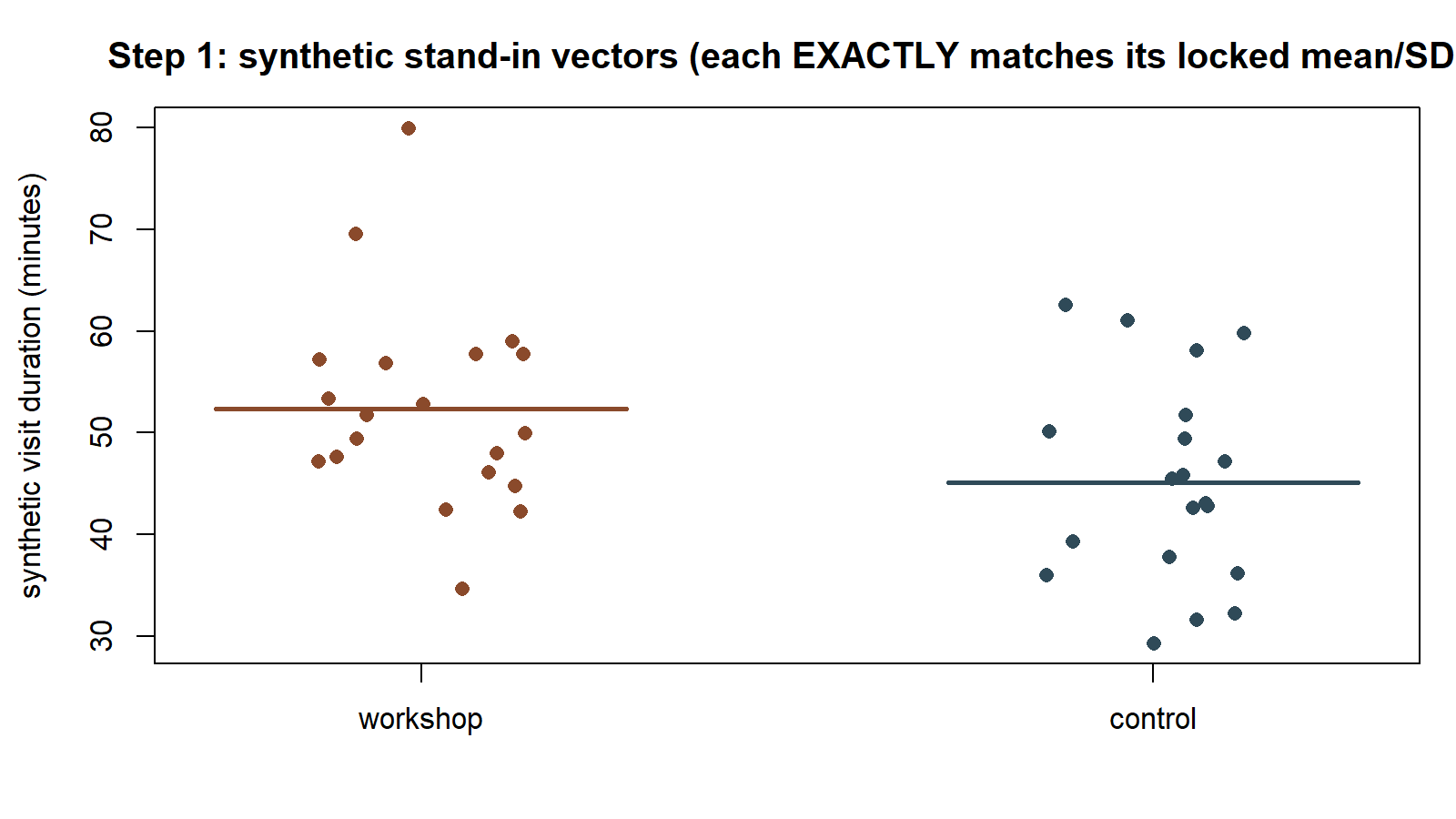
A note on what “synthetic stand-in vectors” means here: the week-11 note works from summary statistics only (n, mean, SD per group), not raw per-student visit times — the raw values were never recorded in this built world. To run an actual permutation test in code, we need 40 individual numbers to shuffle. So this step constructs one synthetic vector of 20 values for each group that exactly reproduces the group’s locked mean and SD, purely as a computational stand-in for “the individual visit-duration values behind the summary.” These constructed numbers are not new data and do not replace the locked summary statistics — they exist only so sample() has 40 concrete values to shuffle.

Steps

Step 1 — Construct synthetic stand-in vectors for each group

The cleanest way to build a vector with an exact target mean and SD (rather than an approximate one from random draws) is to draw a starting sample, then rescale and re-center it so its mean and SD match the target exactly.

set.seed(35103)

make_exact_vector <- function(n, target_mean, target_sd) {
  raw <- rnorm(n)                                   # arbitrary starting draws
  raw_centered <- raw - mean(raw)                    # now has mean exactly 0
  raw_scaled <- raw_centered / sd(raw_centered)       # now has SD exactly 1
  raw_scaled * target_sd + target_mean                # rescale/recenter to target
}

workshop_synth <- make_exact_vector(n_workshop, mean_workshop, sd_workshop)
control_synth  <- make_exact_vector(n_control,  mean_control,  sd_control)

# Sanity check: these are SYNTHETIC STAND-IN values, constructed only to match
# the locked summary statistics exactly -- these are illustrative, not measured values.
mean(workshop_synth); sd(workshop_synth)
mean(control_synth);  sd(control_synth)

Check that mean(workshop_synth) prints 52.4, sd(workshop_synth) prints 10, mean(control_synth) prints 45.1, and sd(control_synth) prints 10 (up to tiny floating-point rounding). If any of these is off, the rescale-and-recenter step above has an error — fix it before moving on, since every later step depends on these two vectors having exactly the right summary statistics.

This chunk is shown but not executed on this page. The figure below was produced by running exactly this chunk’s code separately (same seed 35103), so you can see the two synthetic stand-in vectors as 20 + 20 points rather than only as four summary numbers:

Figure 2: The synthetic stand-in vectors, visualized (synthetic). 20 workshop points and 20 control points, each group constructed to match its locked mean/SD exactly — the short horizontal segments mark each group’s mean (52.4 and 45.1).

Step 2 — Pool the two groups and reshuffle the labels once, by hand

Before automating 5000 shuffles, do one shuffle by hand so you can see exactly what “reshuffle the labels” means at the vector level.

set.seed(35103)

pooled_values <- c(workshop_synth, control_synth)              # all 40 numbers together
group_labels  <- c(rep("workshop", n_workshop), rep("control", n_control))  # the TRUE labels

length(pooled_values)   # should be 40
table(group_labels)     # should be 20 workshop, 20 control

# One random reshuffle of the labels (values stay in place; labels get scrambled):
shuffled_labels <- sample(group_labels)          # sample() with no `size` argument
                                                  # permutes the vector by default
table(shuffled_labels)   # still 20 and 20 -- shuffling a label vector preserves
                          # the group sizes, it just scrambles WHICH value gets WHICH label

# Mean difference under this one shuffle:
shuffled_diff <- mean(pooled_values[shuffled_labels == "workshop"]) -
                 mean(pooled_values[shuffled_labels == "control"])
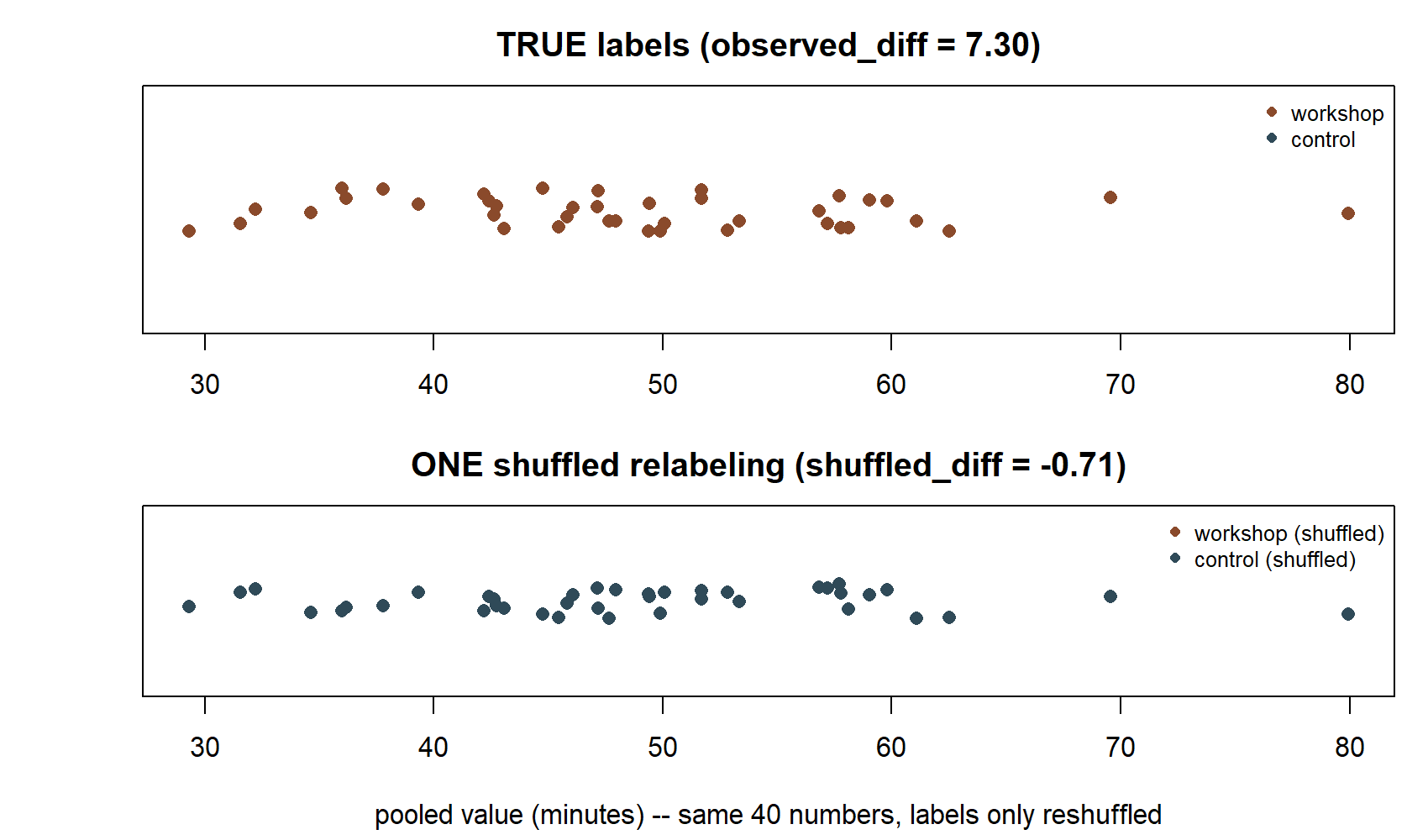
shuffled_diff

Notice what changed and what didn’t: pooled_values never moves — it is the same 40 numbers in the same order throughout. Only group_labels gets shuffled by sample(). This is the entire mechanical content of a permutation test: re-deal which value gets which label, assuming the null hypothesis that the label carries no real information about the outcome. Run this chunk a few times without the set.seed() line (or with a different seed) and watch shuffled_diff bounce around near 0 — under the null, a random relabeling should produce a mean difference centered near zero, unlike the observed 7.3.

This chunk is shown but not executed on this page. The figure below was produced by running exactly this chunk’s code separately (same seed 35103), stacking the true labeling and one shuffled relabeling of the same 40 pooled values so the mechanics are visible:

Figure 3: One shuffle, before and after (synthetic). The same 40 pooled values, first colored by their TRUE workshop/control labels (top, difference 7.3), then by ONE random relabeling (bottom, difference −0.71 for this particular shuffle) — the values never move; only which color each point gets changes.

Step 3 — Automate the shuffle with replicate() to build the permutation null distribution

Now repeat Step 2’s single shuffle B = 5000 times, saving the mean difference from every shuffle, using replicate().

set.seed(35103)

B <- 5000  # number of random permutations

permutation_diffs <- replicate(B, {
  shuffled_labels <- sample(group_labels)
  mean(pooled_values[shuffled_labels == "workshop"]) -
    mean(pooled_values[shuffled_labels == "control"])
})

length(permutation_diffs)   # should be 5000
mean(permutation_diffs)     # should be close to 0 -- the null-distribution center
sd(permutation_diffs)       # the permutation "standard error" of the mean difference

hist(permutation_diffs,
     breaks = 40,
     main = "Permutation null distribution of the mean difference\n(workshop label shuffled 5000 times)",
     xlab = "Shuffled mean difference (workshop - control)")
abline(v = observed_diff, col = "red", lwd = 2)
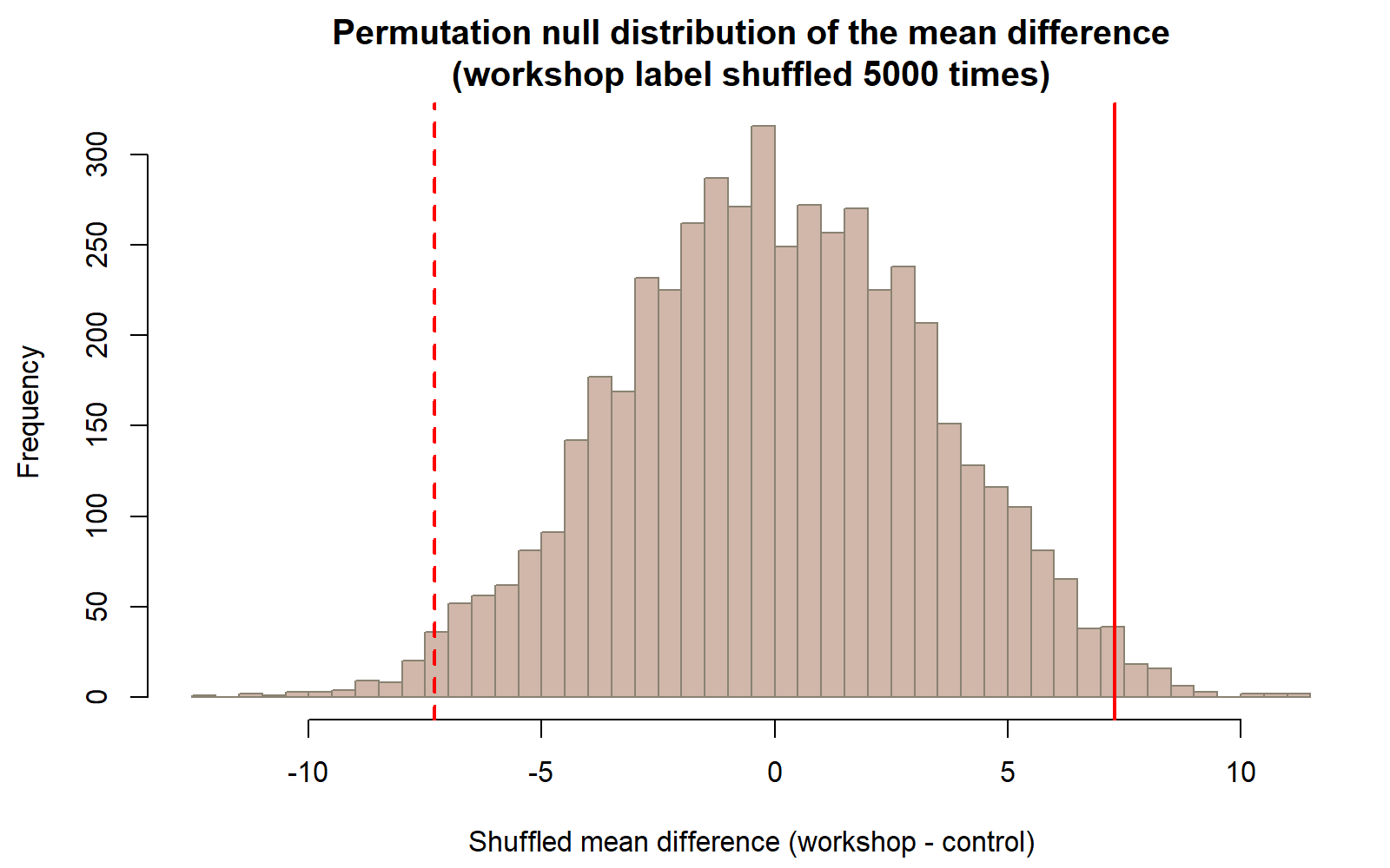
abline(v = -observed_diff, col = "red", lwd = 2, lty = 2)

mean(permutation_diffs) should land close to 0 (it will not be exactly 0, since it’s built from a finite number of random shuffles), confirming that under label-shuffling alone, the “typical” mean difference is near zero — very different from the actually observed 7.3. The two vertical red lines mark ±7.3, the observed difference and its mirror image, so you can see visually how far into the tail(s) the observed value sits relative to the bulk of the shuffled differences.

This chunk is shown but not executed on this page (eval: false) — running it yourself is the point. The figure below was produced by running exactly this chunk’s hist()/abline() code separately (same seed, same B = 5000), so you can check your prediction of its shape against a real result:

Figure 4: The permutation null distribution, rendered (synthetic). A histogram of 5000 shuffled mean differences, centered near 0, with solid/dashed lines at ±7.3 marking the observed difference and its mirror image — the observed value sits visibly out in the tail of this purely label-shuffled world.

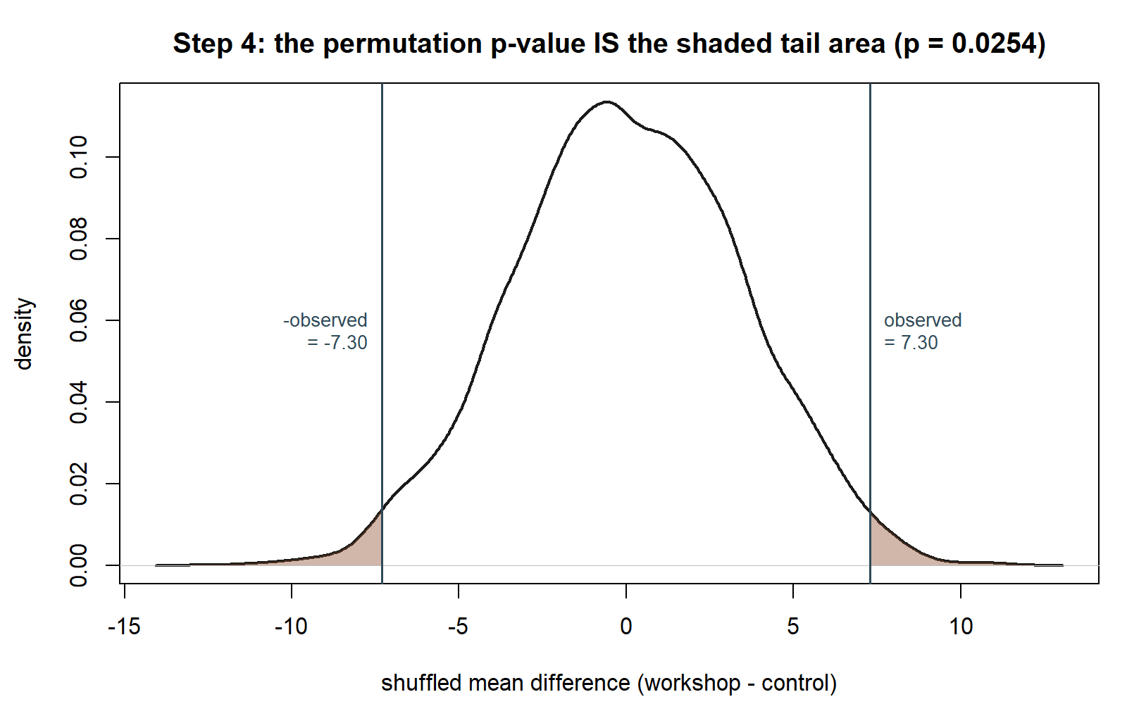
Step 4 — Compute the two-sided permutation p-value

The permutation p-value is the proportion of shuffled mean differences that are at least as extreme as the observed difference, in either direction (two-sided, matching the week note’s two-sided z-test).

set.seed(35103)

# Re-run so this chunk is self-contained if executed on its own:
permutation_diffs <- replicate(B, {
  shuffled_labels <- sample(group_labels)
  mean(pooled_values[shuffled_labels == "workshop"]) -
    mean(pooled_values[shuffled_labels == "control"])
})

# Two-sided: count shuffles at least as extreme (in absolute value) as the observed difference.
permutation_p_value <- mean(abs(permutation_diffs) >= abs(observed_diff))
permutation_p_value

mean(abs(permutation_diffs) >= abs(observed_diff)) is doing two things worth spelling out. First, abs(permutation_diffs) >= abs(observed_diff) produces a vector of 5000 TRUE/FALSE values, one per shuffle, TRUE exactly where that shuffle’s mean difference was at least as far from 0 (in either direction) as the observed 7.3. Second, mean() applied to a logical vector treats TRUE as 1 and FALSE as 0, so it returns the proportion of TRUEs — exactly the permutation p-value: the fraction of random relabelings that produced a difference this extreme or more, purely by chance, under the null.

This chunk is shown but not executed on this page. The figure below extends this chunk’s permutation_p_value with a shaded-tail plot not written on the page, produced by running exactly this chunk’s code separately (same seed, same B = 5000) — the same “p-value IS the shaded area” idea used elsewhere in this course, applied here to a simulated rather than a formula-based null distribution:

Figure 5: The permutation p-value is the shaded tail area (synthetic). A smoothed density of the 5000 shuffled mean differences, with both tails beyond ±7.3 shaded — that shaded area, on both sides combined, IS the two-sided permutation p-value, 0.0254 for this particular run (the week-11 note’s normal-approximation p ≈ 0.021 is close but not identical, as expected from two different, if closely-agreeing, methods).

Verify

Check your work against these three things, in order:

1. Group construction. mean(workshop_synth) = 52.4, sd(workshop_synth) = 10, mean(control_synth) = 45.1, sd(control_synth) = 10, and observed_diff = 7.3 (up to floating-point rounding). If any of these is off, nothing downstream is trustworthy.
2. Null-distribution sanity. mean(permutation_diffs) should be close to 0 and sd(permutation_diffs) should be in the same ballpark as the normal-approximation SE_diff from the week note (SE_diff = sqrt(10²/20 + 10²/20) = sqrt(10) ≈ 3.162) — the permutation approach and the normal-approximation approach are answering the same question two different ways, so their spread estimates should roughly agree.
3. The headline comparison. Your permutation_p_value should land close to the week note’s normal-approximation two-sided p-value of p ≈ 0.021 — not necessarily identical (this is a Monte Carlo estimate from B = 5000 random shuffles, so it carries its own simulation noise), but in the same neighborhood, typically within about 0.005–0.015 of 0.021 across different seeds. This is exactly the agreement the week note predicts: “the permutation p-value is reported as closely matching this approximation (≈ 0.02), as it should when group sizes/spreads are this close to equal.” If your two group sizes are equal (20 and 20, as here) and the spreads are similar (SD = 10 for both), the permutation test and the normal approximation should tell essentially the same story. If your number came out wildly different (say, off by a factor of 5 or more), re-check Steps 1–4 for a labeling or indexing mistake before trusting the result.

As a final gut-check, increasing B (say, to 20000 or 50000) should make permutation_p_value settle down and vary less from run to run — a basic property of Monte Carlo estimation: more replications, less simulation noise, but the same underlying answer.

AI use note

Tool	Purpose	Verification
AI chat assistant (e.g., a general-purpose LLM)	Explaining what replicate() and sample() do in plain language, or suggesting a first draft of the rescale-and-recenter helper function in Step 1	Every suggested line was checked against R’s own documentation (?sample, ?replicate) and against the Verify section’s numeric targets above (exact means/SDs, p-value neighborhood) before being treated as correct; no AI output was accepted without running it and checking it against the locked numbers in this lab and the week-11 note
AI code-completion tool	Autocompleting routine lines (variable names, closing parentheses) while typing the chunks above	Read and re-typed/checked against the intended base-R-only, no-package constraint before accepting; any suggested use of infer, dplyr, or other packages was rejected in favor of the base-R equivalent shown here

The graded deliverable, its rubric, and due date live in Blackboard (the LMS) — this page is study and practice only.

See also

• Week 11 — Randomization and permutation tests — the companion week note; develops the logic of the randomization test and the normal-approximation cross-check (p ≈ 0.021) that this lab’s permutation p-value is compared against.
• Lab 10 — Bootstrap intervals — the previous lab’s resampling technique (resampling within a group with replacement) contrasted with this lab’s resampling technique (shuffling labels across groups without replacement).
• Inference formula reference — the normal-approximation two-sample difference formulas used in the Verify section above.
• R/Quarto setup — how to run these chunks in your own RStudio/Posit Cloud session (recall: chunks in this build are shown with #| eval: false and are meant to be run by you, not executed automatically).