Week 13 — A simulation study of method behavior
Comparing the t-test and Wilcoxon by Monte Carlo: Type I error, power, and Monte Carlo error
Source basis. Original instructor-authored notes; all data is synthetic, generated by a Monte Carlo study with a fixed generator (seed 45213). Open texts are conceptual companions cited by section title only (map-don’t-mine); no prose, figures, examples, or exercises are reproduced. See Open readings & attribution. Ungraded — Blackboard is authoritative for graded work.
This week. For twelve weeks we have chosen methods — permutation, bootstrap, rank, robust. Now we turn the tables and put two methods on trial. When the truth is something we control, we can watch how a method behaves: how often it cries wolf when nothing is happening, and how often it catches a real effect. That is a simulation study, and it is how statisticians actually decide which tool to reach for.
Learning goals
By the end of this week you should be able to:
- Describe the Monte Carlo simulation loop: choose a truth, generate data, apply each method, record, repeat, summarize.
- Estimate a method’s Type I error (rejection rate when the null is true) and its power (rejection rate when a real effect exists), and read them from bar charts and power curves.
- Explain why, under heavy tails, the Wilcoxon test can have more power than the t-test even though both control Type I error.
- Report a Monte Carlo standard error and resist reading a single short run as the answer.
Where we are
A hypothesis test is a decision rule. Feed it data and it says reject or don’t reject. We usually apply it once, to one real dataset, and we never get to see whether it decided well. A simulation study buys back that missing feedback: because we invent the truth, we know the right answer, so we can run the rule thousands of times and simply count how often it is right.
The simulation loop
Every simulation study is the same loop. Pick a data-generating process (a “DGP”) and a true effect size; draw a fresh dataset from it; apply each method and record whether it rejected at \(\alpha = 0.05\); repeat \(B\) times; then summarize the recorded decisions into rates.
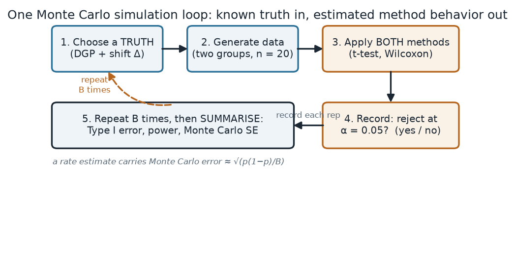
What to notice. Nothing here is a formula for the answer — it is a procedure for estimating one. The truth is our choice (box 1), so we always know whether a rejection was a false alarm or a real catch. Because the summary is a proportion out of \(B\) runs, it is itself an estimate with its own uncertainty (box 5).
The loop, as steps (nonvisual equivalent).
| Step | What happens |
|---|---|
| 1 | Choose the truth: a DGP (Normal or heavy-tailed) and a true shift \(\Delta\) |
| 2 | Generate two groups, \(n = 20\) each |
| 3 | Apply both methods: pooled t-test and Wilcoxon rank-sum |
| 4 | Record: did each reject at \(\alpha = 0.05\)? |
| 5 | Repeat \(B\) times, then summarize: Type I error, power, Monte Carlo SE |
Two truths we can dial in
We use two DGPs, both symmetric so the comparison is fair. The Normal DGP draws each observation from \(N(\mu, 1)\). The heavy-tailed DGP is a contaminated Normal: each observation is drawn from \(N(\mu, 1)\) with probability \(0.90\) and from \(N(\mu, 6^2)\) with probability \(0.10\). It has the same center \(\mu\), but its standard deviation is \(\sqrt{0.9\cdot 1 + 0.1\cdot 36} \approx 2.12\) — most points are ordinary, but roughly one in ten is a wild outlier. Under the null we set the true shift \(\Delta = 0\); under an alternative we shift the second group’s center by \(\Delta\).
The R that runs this is a short loop — and notice there is no plotting in it; the pictures below are downstream summaries:
# One Monte Carlo study: t-test vs Wilcoxon, two-sided, alpha = 0.05
set.seed(45213)
n <- 20; alpha <- 0.05; B <- 8000

# a contaminated-Normal draw: N(mu,1) w.p. 0.9, N(mu,6^2) w.p. 0.1
draw_heavy <- function(n, mu) {
  big <- runif(n) < 0.10
  rnorm(n, mean = mu, sd = ifelse(big, 6, 1))
}

one_rep <- function(shift) {                 # TRUE/FALSE rejection for each method
  x <- draw_heavy(n, 0)
  y <- draw_heavy(n, shift)
  c(t   = t.test(x, y, var.equal = TRUE)$p.value < alpha,
    wil = wilcox.test(x, y)$p.value            < alpha)
}

rej <- replicate(B, one_rep(shift = 0))       # Type I error: no true difference
rowMeans(rej)                                 # estimated Type I error, per method
sqrt(rowMeans(rej) * (1 - rowMeans(rej)) / B) # Monte Carlo standard error
Worked example — Type I error: a fair false-alarm rate?
First we hold the null true (\(\Delta = 0\)) and ask how often each test rejects anyway. That rate should be close to the target \(\alpha = 0.05\). We run \(B = 8000\) replications in each of the two DGPs.
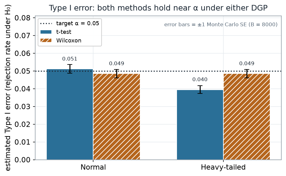
What to notice. Both tests keep their false-alarm rate near \(0.05\) under either DGP — the t-test is not “broken” by heavy tails here; if anything it becomes slightly conservative (0.040), rejecting a touch less often than advertised. The headline is what this rules out: since Type I error is controlled for both, the choice between them cannot be settled here. It has to be decided on power.
Type I error read-out (nonvisual equivalent).
| Data (DGP) | t-test | Wilcoxon | MC SE (t-test) | MC SE (Wilcoxon) |
|---|---|---|---|---|
| Normal | 0.051 | 0.049 | ≈ 0.0025 | ≈ 0.0024 |
| Heavy-tailed | 0.040 | 0.049 | ≈ 0.0022 | ≈ 0.0024 |
| Target \(\alpha\) | 0.050 | 0.050 | — | — |
Worked example — power under heavy tails
Now we make the alternative true: we shift the second group by a real amount \(\Delta\) and ask how often each test catches it. Sweeping \(\Delta\) from \(0\) to \(2\) traces a power curve for each method under the heavy-tailed DGP (\(B = 4000\) per point).
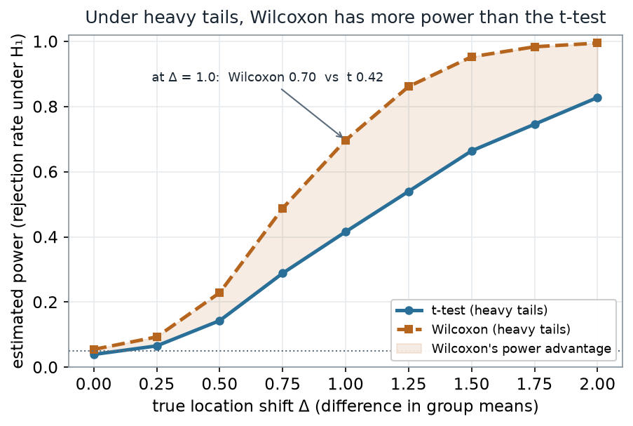
What to notice. Same data, same \(\alpha\), very different power. The ten-percent outliers inflate the t-test’s pooled standard deviation, which shrinks its signal-to-noise ratio and costs it rejections. Wilcoxon works on ranks, so a wild outlier is just “the largest value” and carries no extra leverage. The gap is widest near \(\Delta = 1.25\), where Wilcoxon reaches \(0.86\) and the t-test only \(0.54\).
This is not a universal verdict. Re-run the same sweep on the clean Normal DGP and the ranking nearly reverses: at \(\Delta = 0.75\) the t-test’s power is \(0.643\) and Wilcoxon’s is \(0.610\) — the t-test is slightly ahead when its assumptions hold. The lesson is conditional: Wilcoxon buys robustness to heavy tails, and pays a small efficiency tax when the data is well-behaved.
Power read-out under heavy tails (nonvisual equivalent).
| True shift \(\Delta\) | t-test | Wilcoxon |
|---|---|---|
| 0.50 | 0.143 | 0.229 |
| 0.75 | 0.288 | 0.488 |
| 1.00 | 0.416 | 0.697 |
| 1.25 | 0.540 | 0.862 |
| 1.50 | 0.664 | 0.953 |
How much can we trust one run?
Every rate above is an estimate from a finite number of replications, so it wobbles. To see how much, watch the running estimate of the t-test’s Normal-null Type I error as replications accumulate. The true value is exactly \(0.05\) (the t-test is exact under Normality), and the shaded band is \(\pm 2\) Monte Carlo standard errors, \(\pm 2\sqrt{0.05\cdot 0.95 / B}\), around that truth.
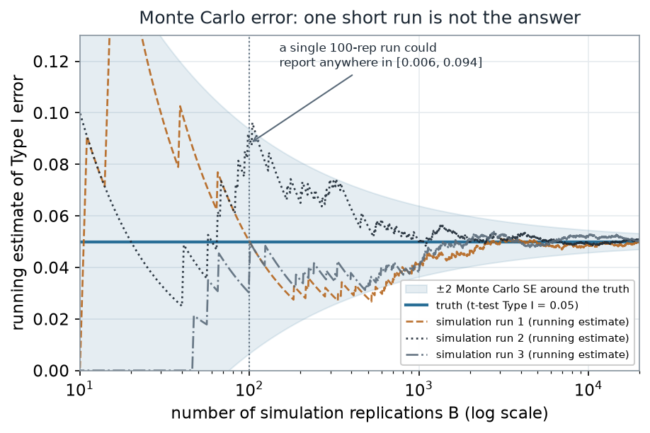
What to notice. Early on, the three runs disagree wildly — a \(100\)-replication study of a true-\(0.05\) rate could land almost anywhere from under \(1\%\) to over \(9\%\). Only as \(B\) climbs do they funnel onto the truth. To halve the Monte Carlo error you must quadruple \(B\). A reported simulation rate without a Monte Carlo SE is a number without its own error bar.
Monte Carlo error read-out (nonvisual equivalent).
| Replications \(B\) | \(\pm 2\) Monte Carlo SE band around 0.05 |
|---|---|
| 100 | [0.006, 0.094] |
| 1000 | [0.036, 0.064] |
| 10000 | [0.046, 0.054] |
| 20000 (final estimate) | reported 0.0496 |
A common mistake
“The simulation said Wilcoxon rejects 70% of the time, so that’s the power.” One run is not the truth — it is a draw from a distribution centered near the truth with spread \(\sqrt{p(1-p)/B}\). Read a single short simulation as the answer and you are quoting a noisy estimate to three decimals. Always report the Monte Carlo standard error, make \(B\) large enough that it is small relative to the differences you care about, and remember that every result is conditional on the DGP you chose — change the truth and the ranking of methods can change with it.
Check your understanding (ungraded)
- In your own words, what is the difference between Type I error and power, and why do we hold \(\Delta = 0\) to estimate one and set \(\Delta \ne 0\) to estimate the other?
- Under heavy tails the t-test’s Type I error was \(0.040\) — slightly below \(0.05\). Does being conservative on Type I error help or hurt its power, and how does the power figure bear that out?
- A classmate runs \(200\) replications and reports a power of “\(0.685\)”. Using \(\sqrt{p(1-p)/B}\), roughly how wide is the \(\pm 2\) Monte Carlo SE interval, and what would you tell them?
- The Normal-DGP sweep put the t-test slightly ahead of Wilcoxon. Explain why “which test is more powerful?” has no answer until you say what the data-generating process is.
Reading guide
- IMS — Decision errors (Type I and Type II) — a conceptual companion to the two error rates our study estimates; read it for the definitions, then verify them against the bar chart above.
- Learning Statistics with R (Navarro) — Comparing two means and The Wilcoxon test — background on the two methods we put on trial (cited, not reproduced).
- NIST/SEMATECH e-Handbook — Assessing the power of a test — an instructor reference for framing power as something we can estimate by simulation.
- ModernDive — Hypothesis testing (simulation-based) — reinforces the simulate-and-count logic that the Monte Carlo loop generalizes.
Accessibility notes
Mathematics is live text (\(\sqrt{p(1-p)/B}\) renders as MathML, not an image). Every figure carries an alt line stating its message, a “what to notice” reading, and an adjacent data-summary table, so each point survives without the picture. Series are distinguished by linestyle, hatch, and marker (t-test = solid/circles, Wilcoxon = dashed-or-hatched/squares) plus value-bearing labels, never color alone. The running-estimate trajectories use three distinct dash styles. A clean lint and a clean render are evidence; the rendered assistive-technology review is a human step.
Assessment (descriptive only)
This week contributes learning evidence toward designing a small simulation study and reading Type I error, power, and Monte Carlo error to compare methods. That is the shape only; the actual graded prompts, weights, and due dates live in Blackboard.
Public vs. graded. These are public, ungraded notes and practice. Graded prompts, keys, rubrics, point values, and due dates live in Blackboard Ultra, which governs.
Looking ahead
Next week we stop testing methods against invented truths and start applying them to a case: an applied robust-methods report that reads a dataset’s structure, names what is fragile, runs two methods, checks sensitivity, and reports honestly — the shape your project will take.