Week 12 — Comparing parametric, rank-based, and resampling methods
One comparison, three lenses — and what to do when they disagree
Source basis. Original instructor-authored notes; all data is synthetic (two groups of “response minutes”, generated from a fixed generator, seed 45212). Open texts are conceptual companions cited by section title only (map-don’t-mine); no prose, figures, examples, or exercises are reproduced. See Open readings & attribution. Ungraded — Blackboard is authoritative for graded work.
This week. We have built three ways to compare two groups: a t-test (a parametric statement about the difference in means), a Wilcoxon rank-sum test (a distribution-free statement about a shift), and a bootstrap interval (a resampling statement about the difference in means). This week we put all three on the same comparison and ask the real question: when do they agree, when do they diverge, and what does a divergence tell you?
Learning goals
By the end of this week you should be able to:
- Run a two-sample t-test, a Wilcoxon / Hodges–Lehmann shift, and a bootstrap interval on one comparison, and read all three as intervals for “the effect.”
- Recognize that on clean, near-normal data the three methods roughly agree, so the choice barely matters.
- Explain why they diverge on skewed data with outliers — and trace the split to the estimand (mean vs shift), not merely to “parametric vs nonparametric.”
- Report a divergence honestly instead of cherry-picking the method that reaches significance.
Where we are
Every method this term has been a different answer to what is fragile here, and what can we still say? Now we hold the data fixed and vary the method. The comparison is always the same: a location effect, group B minus group A, in response minutes. Three lenses look at it:
- Two-sample t — targets the difference in means; a normal-theory interval \(\bar x_B-\bar x_A \pm t_{\,0.975}\,\widehat{\mathrm{SE}}\).
- Wilcoxon rank-sum / Hodges–Lehmann — targets a location shift; the estimate is the median of all pairwise differences \(b_j - a_i\), with a distribution-free interval.
- Bootstrap (percentile) — targets the difference in means again, but builds its interval by resampling rather than by a normal formula.
When the data is clean, the three agree
Our first cohort is near-normal: two symmetric groups (\(n_A = n_B = 24\)) with a real separation. Group A sits near 52 minutes, group B near 60. Here is the effect, estimated three ways.
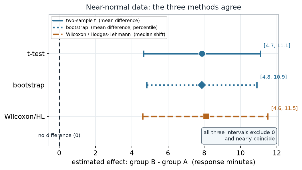
What to notice. The three intervals sit almost on top of one another, all comfortably to the right of zero. On clean, symmetric data the mean difference and the median shift describe the same thing, and the normal formula, the rank method, and the resample all land in the same place. Here the choice of method is almost a matter of taste.
The three effect estimates, near-normal cohort (nonvisual equivalent).
| Method (near-normal) | Effect estimate | 95% interval | p-value | excludes 0? |
|---|---|---|---|---|
| Two-sample t (mean difference) | 7.9 | [4.7, 11.1] | < 0.001 | yes |
| Bootstrap (mean difference) | 7.9 | [4.8, 10.9] | — | yes |
| Wilcoxon / Hodges–Lehmann (shift) | 8.1 | [4.6, 11.5] | < 0.001 | yes |
Add skew and two outliers
Now a second cohort of the same size, with a similarly clear bulk separation — the realized rank shift is again about 7–8 minutes — but the measurements are right-skewed, and group A picks up two extreme values (118 and 132 minutes: a timer left running). The genuine bulk separation is still there; only the shape of the data, and the two outliers, is new. Watch what happens to the three intervals.
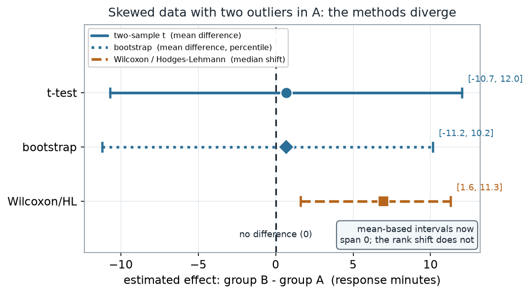
What to notice. The mean-based intervals — both the t and the bootstrap — collapsed toward zero and now include it (t: p = 0.90). The rank-based shift barely moved and stays significant (p = 0.01). The two mean-based methods agree with each other and disagree with the rank method: the split is about what is being estimated, not about a formula versus a resample.
The three effect estimates, skewed cohort (nonvisual equivalent).
| Method (skewed + 2 outliers) | Effect estimate | 95% interval | p-value | excludes 0? |
|---|---|---|---|---|
| Two-sample t (mean difference) | 0.7 | [−10.7, 12.0] | 0.90 | no |
| Bootstrap (mean difference) | 0.7 | [−11.2, 10.2] | — | no |
| Wilcoxon / Hodges–Lehmann (shift) | 7.0 | [1.6, 11.3] | 0.01 | yes |
Why they split
The divergence is not mysterious once you look at the data. The two outliers do two things to the mean difference: they drag group A’s mean up until it nearly matches group B’s, and they inflate the standard error until the interval is enormous. The ranks — and the median-of-pairwise shift — never feel the outliers’ magnitude, only their order, so they keep reporting the bulk separation.
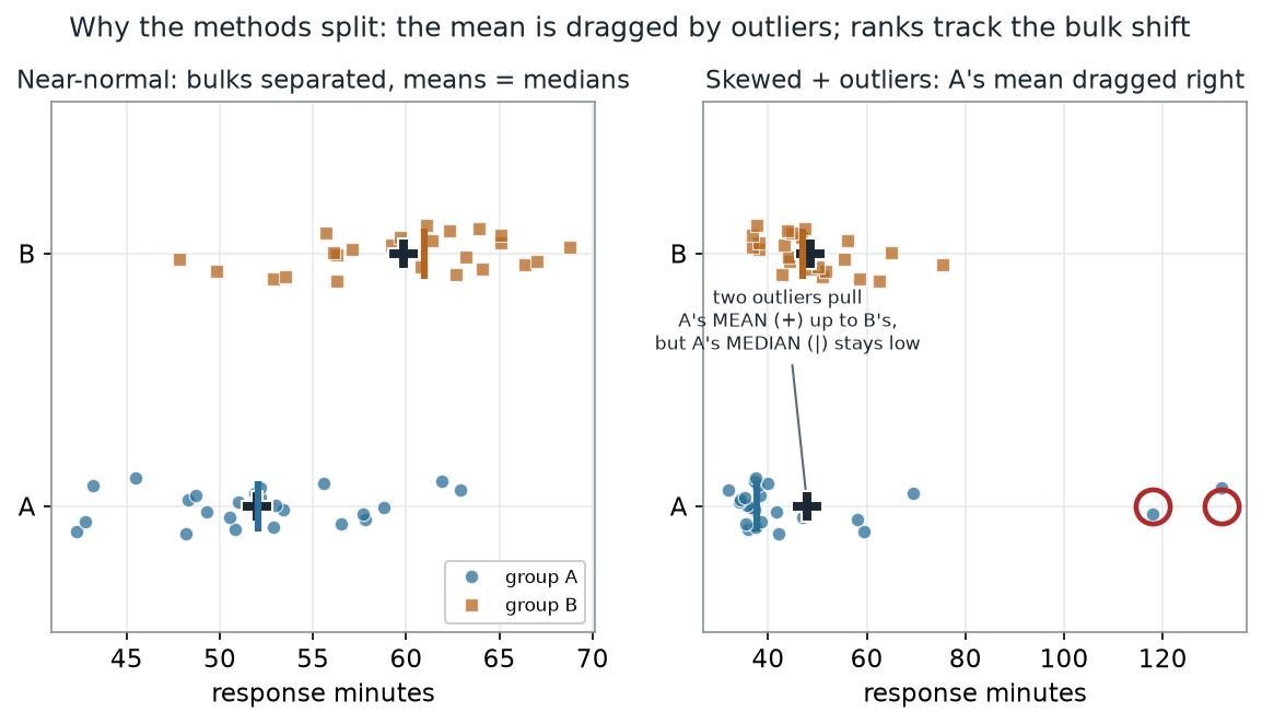
What to notice. In the skewed panel, group A’s median (37.7) sits far below group B’s (47.1) — the bulk shift the rank test reports. But A’s mean is pulled up to 48.0, essentially equal to B’s 48.6. Remove A’s two outliers and its mean drops back to 41.0. The mean and its interval are doing exactly what a mean does near heavy tails; the ranks are doing exactly what ranks do.
The two cohorts as group summaries (nonvisual equivalent).
| Skewed-cohort summary | Group A | Group B |
|---|---|---|
| Mean | 48.0 | 48.6 |
| Mean without A’s two outliers | 41.0 | 48.6 |
| Median | 37.7 | 47.1 |
| The two outliers in A | 118, 132 | — |
Means are shown to one decimal place; the mean difference reported above (0.7) is computed from the unrounded means (47.96 and 48.64, a difference of 0.68), so it need not equal the difference of the rounded values shown here (48.6 − 48.0 = 0.6).
Worked example — the skewed comparison, step by step
Take the skewed cohort and run all three analyses. The R is short, and notice there is no plotting in it — the pictures above are the downstream evidence:
# Schematic: the named data objects are the sample(s) described in the text above; this illustrates the analysis, not a self-contained runnable block.
# one comparison, three lenses (response minutes for group A vs group B)
t.test(response ~ group, data = d)                        # Welch t: mean difference + 95% CI
wilcox.test(response ~ group, data = d, conf.int = TRUE)  # rank-sum p + Hodges-Lehmann shift + CI

# bootstrap the MEAN difference, percentile interval (no plotting call)
set.seed(45212)
B    <- 4000
diff <- replicate(B, {
  a <- sample(d$response[d$group == "A"], replace = TRUE)
  b <- sample(d$response[d$group == "B"], replace = TRUE)
  mean(b) - mean(a)
})
quantile(diff, c(0.025, 0.975))
Reading the output the way a report should:
- The t-test returns a mean difference of 0.7 minutes, 95% CI [−10.7, 12.0], p = 0.90. Taken alone, this says “no detectable difference.” But the interval is nearly 23 minutes wide — the test is not confident of nothing; it is uninformative, because the outliers blew up the standard error.
- The bootstrap of the mean difference agrees: 0.7, percentile interval [−11.2, 10.2]. This is the crucial subtlety — the bootstrap is a nonparametric method, yet it also crosses zero. It inherits the fragility of its estimand: it is still estimating the mean difference, and the mean is what the outliers wreck.
- The Wilcoxon / Hodges–Lehmann shift is 7.0 minutes, 95% CI [1.6, 11.3], p = 0.01. It targets a shift read from ranks, so the two outliers move it hardly at all, and it detects the bulk separation the mean-based methods miss.
The honest one-paragraph conclusion is not “the groups differ” or “the groups don’t.” It is: the typical (median) response in group B is about 7 minutes longer than in group A, and that shift is well established; the difference in means is not estimable with any precision here because two extreme values dominate it. That sentence reports which estimand is trustworthy and why — which is the whole job.
Reading a divergence honestly
When the methods split, the temptation is to treat them as a menu and keep the result you like. Resist it.
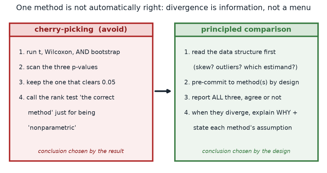
What to notice. “Nonparametric” is not a synonym for “correct.” The bootstrap here was nonparametric and still crossed zero; the rank test won not because it is distribution-free but because its estimand (a shift) is the one the outliers cannot corrupt. Pick the method for what it estimates and how the data is shaped, before you see which p-value clears the line.
The two habits (nonvisual equivalent).
| Habit | What drives the conclusion |
|---|---|
| Cherry-picking (avoid) | the single p-value that happens to clear 0.05 |
| Principled comparison | data structure + a pre-committed design; report all three and explain the split |
“When methods disagree, the nonparametric one is the right answer.” Not automatically. The right method is the one whose estimand and assumptions match your question and your data — decided before you peek at significance. On the skewed cohort the rank test was more informative because a median shift resists outliers, not because “nonparametric” is a magic word; the nonparametric bootstrap of the mean failed right alongside the t-test. And when all three agree, as in the clean cohort, no cherry-picking is even possible — which is exactly why you report all three.
Check your understanding (ungraded)
- On the near-normal cohort the three intervals nearly coincided; on the skewed cohort the t and bootstrap crossed zero while Wilcoxon did not. In one sentence, what changed — the method or the data?
- The bootstrap is a nonparametric, resampling method, yet its interval crossed zero on the skewed cohort. Explain why being “nonparametric” did not protect it.
- Group A’s mean was 48.0 with the two outliers and 41.0 without them, while its median was 37.7. Which estimand would you report for this cohort, and how would you justify it?
- A colleague runs t, Wilcoxon, and bootstrap, then reports only the one with p < 0.05. Name two things wrong with that habit, and state what they should have done first.
Reading guide
- OpenIntro Statistics 4e — Inference for comparing two independent means — the parametric baseline the t interval rests on; read for the mean-difference framing.
- IMS — Comparing two means / mathematical vs simulation-based inference — reinforces that the same comparison can be approached by a formula or by resampling.
- Learning Statistics with R (Navarro) — The Wilcoxon rank-sum test — an instructor reference for the rank-based shift and when to prefer it (cited, not reproduced).
- ModernDive — Bootstrapping and confidence intervals — the resampling interval as a distribution-free alternative to the t interval, and its limits.
Accessibility notes
Mathematics is live text (\(\bar x_B - \bar x_A \pm t_{0.975}\,\widehat{\mathrm{SE}}\) renders as MathML, not an image). Every figure carries an alt line stating its message, a “what to notice” reading, and an adjacent data-summary table, so each point survives without the picture. The three methods are distinguished by linestyle and marker (t = solid circle, bootstrap = dotted diamond, Wilcoxon/HL = dashed square) and by value-bearing labels, not color alone; the two-habit diagram is distinguished by its heading labels (“cherry-picking (avoid)” vs “principled comparison”) and footers, not color. A clean lint and a clean render are evidence; the rendered assistive-technology review is a human step.
Assessment (descriptive only)
This week contributes learning evidence toward running a comparison three ways and reading agreement or divergence and choosing a method by estimand and data structure rather than by significance. That is the shape only; the actual graded prompts, points, and due dates live in Blackboard.
Public vs. graded. These are public, ungraded notes and practice. Graded prompts, keys, rubrics, point values, and due dates live in Blackboard Ultra, which governs.
Looking ahead
We have seen that the methods diverge on one skewed cohort. Next week we ask how often and by how much across many datasets: a simulation study that pits the t-test against Wilcoxon under a normal null and a heavy-tailed null, estimating Type I error and power — turning this week’s single side-by-side into a repeatable measurement of method behavior.