Week 9 — Categorical & ordinal outcomes
Small tables, exact tests, and using the order you were handed
Source basis. Original instructor-authored notes; data is synthetic (46 individual ordinal outcomes drawn from a fixed generator, seed 45209, then tabulated). Open texts are conceptual companions cited by section title only (map-don’t-mine); no prose, figures, examples, or exercises are reproduced. See Open readings & attribution. Ungraded — Blackboard is authoritative for graded work.
This week. Our rank methods (weeks 7–8) turned numbers into their order. This week the outcome arrives as categories — sometimes ordered (none < mild < moderate < severe), sometimes not — and the counts are small. We ask two questions: when is the familiar chi-square approximation trustworthy, and how much do we throw away when we treat an ordered outcome as if the categories had no order?
Learning goals
By the end of this week you should be able to:
- Read a contingency table as within-group proportions and describe how two groups differ.
- Explain why the chi-square test is an approximation, and use an exact / permutation null when expected counts are small.
- Contrast a nominal (unordered) test with an ordinal-aware trend test, and say why the trend test can detect a shift the nominal test spreads too thin to see.
- Recognize the mistake of averaging ordinal codes as if they were interval measurements.
Where we are
Every method this term has asked what is fragile here, and what can we still say? For a category count, the fragile move is the approximation: the chi-square test replaces a messy discrete reference distribution with a smooth curve that is only trustworthy when the counts are large enough. And for an ordered outcome, the fragile move is throwing the ordering away — running a test that would give the same answer if you shuffled “mild” and “severe.”
The two-group ordinal outcome
Our running example is a synthetic study: a symptom recorded as none / mild / moderate / severe for two small groups, Control (n = 24) and Treatment (n = 22). The whole dataset is a 2×4 table of counts, and the first honest thing to do is turn it into within-group proportions so the two groups are comparable despite different sizes.
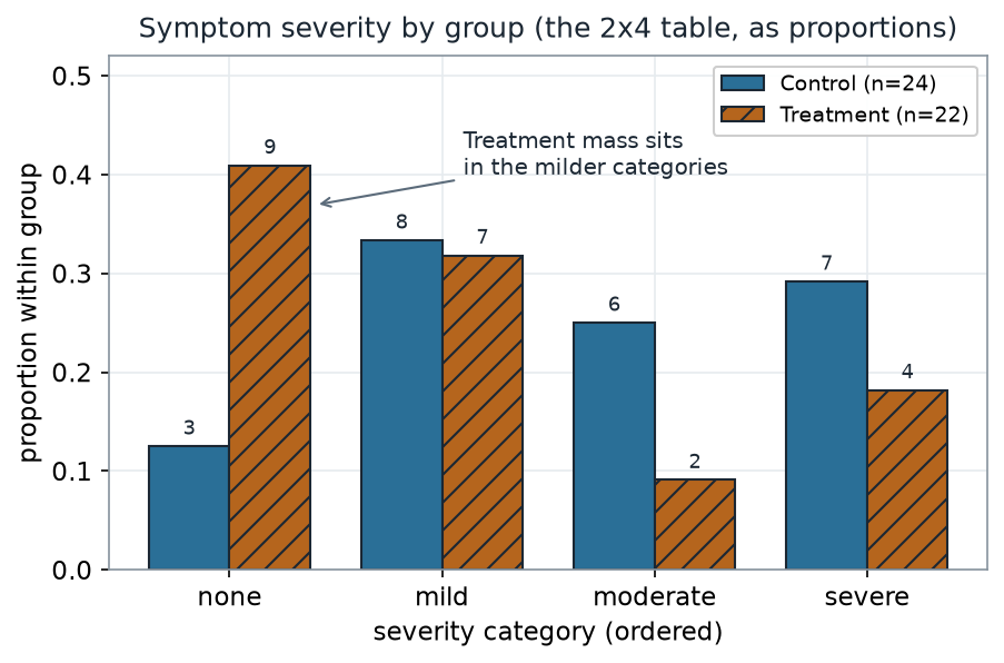
What to notice. Treatment piles up in none/mild; Control carries more moderate/severe. The two groups clearly differ, and — because the categories are ordered — they differ in a directional way: Treatment is shifted toward the mild end. Hold onto that direction; a nominal test will ignore it.
The table, as numbers (nonvisual equivalent).
| Group | none | mild | moderate | severe | n |
|---|---|---|---|---|---|
| Control | 3 | 8 | 6 | 7 | 24 |
| Treatment | 9 | 7 | 2 | 4 | 22 |
| Column total | 12 | 15 | 8 | 11 | 46 |
When the chi-square shortcut gets shaky
Pearson’s chi-square test compares each observed count to the count you’d expect if group and category were unrelated, \(E_{ij} = (\text{row}_i \times \text{col}_j)/N\), and sums \(\sum (O-E)^2/E\). That sum only approximately follows a chi-square curve, and the approximation leans on every expected count being large enough (a common rule of thumb is \(E_{ij} \geq 5\)). Here the smallest expected count is 3.8 — just under the rule — so we should not simply trust the curve. We can instead build the exact reference distribution the way we built permutation nulls in weeks 3–4: hold both margins fixed and re-shuffle which subjects belong to which group.
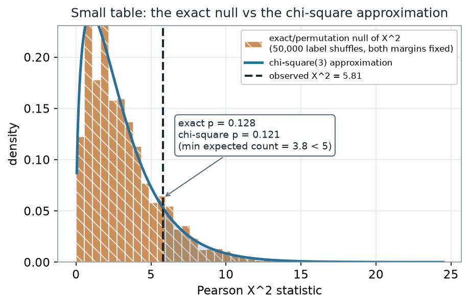
What to notice. The exact null (hatched bars) and the chi-square curve nearly coincide, so here the two p-values almost agree: 0.128 (exact) vs 0.121 (chi-square). That agreement is reassurance, not luck — with a smallest expected count of only 3.8 we were right to check. The lesson is the habit, not the gap: the permutation null always holds; the curve is an approximation you verify. When cells are sparser, the two can diverge sharply, and then the exact answer is the one to report.
Exact vs approximate (nonvisual equivalent).
| Reference for X² = 5.81 | p-value |
|---|---|
| Exact / permutation null (50,000 shuffles, margins fixed) | 0.128 |
| Chi-square(3) approximation | 0.121 |
| Smallest expected count in the table | 3.8 |
Worked example — let the ordering do the work
Both p-values above sit near 0.12 — not significant at the conventional 0.05 line. But that nominal chi-square test asked only “are the groups different somehow?” and split its evidence across 3 degrees of freedom, one for each way the four categories could rearrange. Our groups do not differ in some arbitrary way; Treatment is shifted toward milder severity. A test that uses the order concentrates all its evidence on that single monotone direction.
The linear-by-linear trend test does exactly that: score the ordered categories \(1,2,3,4\), correlate those column scores with the group label across all 46 subjects, and refer \(M^2 = (N-1)\,r^2\) to a chi-square with 1 degree of freedom.
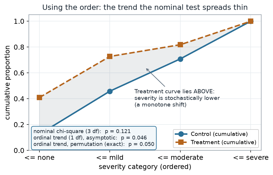
What to notice. The Treatment cumulative curve lies entirely above Control — a clean picture of stochastic ordering (Treatment reaches high cumulative proportion in the mild categories, so it is less severe). Using that order, the trend test concentrates the evidence and moves the p-value from the nominal 0.121 down to 0.046 on a single df. But the rule this week keeps repeating — verify the curve against the exact null — applies to the trend test too: its permutation (exact) p is 0.050, sitting right on the 0.05 line rather than clean below it. Same data, same table — the ordinal test refuses to waste evidence, and the exact reference the week champions calls the trend marginal (≈ 0.05), not decisively significant.
Two tests, one table (nonvisual equivalent).
| Test | Uses the order? | df | Asymptotic p | Permutation (exact) p |
|---|---|---|---|---|
| Nominal chi-square | no | 3 | 0.121 | 0.128 |
| Linear-by-linear trend | yes | 1 | 0.046 | 0.050 |
The asymptotic trend p dips just under 0.05, but its exact permutation analog is 0.050 — on the line, not below it. The honest headline is that the ordinal test concentrates the evidence (0.121 → ≈ 0.05), turning a diffuse non-result into a marginal one; it does not manufacture a clean rejection.
The teaching code is short, and note there is no plotting in it — the pictures above are the output:
# Schematic: the named data objects are the sample(s) described in the text above; this illustrates the analysis, not a self-contained runnable block.
# severity as an ORDERED factor; group is a two-level factor
sev <- factor(severity, levels = c("none", "mild", "moderate", "severe"), ordered = TRUE)
tab <- table(group, sev)             # the 2x4 contingency table
prop.table(tab, margin = 1)          # within-group proportions

# nominal (unordered) test + its small-count exact companion
chisq.test(tab)                      # chi-square approximation (3 df)
fisher.test(tab)                     # Fisher-Freeman-Halton exact test (~0.135 here) -- a DIFFERENT
                                     # exact test from the X^2-permutation p = 0.128 reported above

# ordinal-aware trend: score the columns 1..4 and correlate with the group
u  <- as.integer(sev)                # column scores 1,2,3,4
g  <- as.integer(factor(group))      # row scores
M2 <- (length(u) - 1) * cor(g, u)^2  # linear-by-linear statistic
1 - pchisq(M2, df = 1)               # trend p-value on 1 df
What to notice. Two different “exact” tools. The 0.128 reported above is the permutation null of Pearson’s X² — reshuffle the group labels with both margins fixed, exactly the reference in the exact-vs-approximate table. fisher.test(tab) instead runs the Fisher–Freeman–Halton exact test, a distinct exact procedure that returns ≈ 0.135 on this table. Both are legitimate exact references and they agree to about 0.13 here, but they are not the same computation — so do not expect fisher.test to reproduce the 0.128 to the last digit.
Choosing the test
The week collapses to one decision. Is the outcome a category? Then ask the single question that changes everything: are the categories ordered?
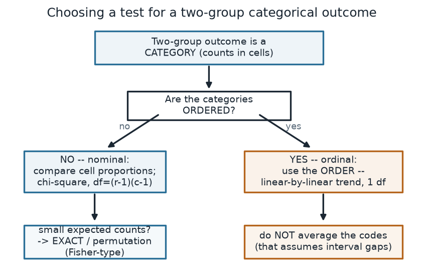
What to notice. The branch you take is a modeling choice about the outcome’s scale, made before you see a p-value — not a search for the smallest number. If the categories are unordered, compare proportions with chi-square and switch to an exact/permutation reference when expected counts are small. If they are ordered, spend your evidence on the trend, and do not collapse the categories to an average.
The decision, as steps (nonvisual equivalent).
| If the outcome is… | Then use… | Small counts? |
|---|---|---|
| Unordered (nominal) categories | Chi-square on the table, df = (r−1)(c−1) | Switch to exact / permutation |
| Ordered (ordinal) categories | Linear-by-linear trend test, 1 df | Permutation trend still valid |
A common mistake — treating ordinal codes as interval
“The categories are coded 1, 2, 3, 4, so just average them and compare the means.” Those codes are labels for an order, not measurements on a scale. Nothing says the step from mild to moderate is the same size as the step from moderate to severe. The moment you average, you have invented those gaps — and a different, equally defensible coding gives a different answer.
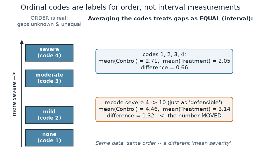
What to notice. With codes \(1,2,3,4\) the “mean severity” gap between groups is 0.66. Recode severe as 10 instead of 4 — just as arbitrary — and the same subjects now give a gap of 1.32. The number moved because it was never anchored to a real unit. The ordering is trustworthy; the spacing is your assumption, so lean on the trend test, which uses only the order.
Coding-dependence (nonvisual equivalent).
| Coding of the four categories | Mean(Control) | Mean(Treatment) | Difference |
|---|---|---|---|
| 1, 2, 3, 4 | 2.71 | 2.05 | 0.66 |
| 1, 2, 3, 10 | 4.46 | 3.14 | 1.32 |
Check your understanding (ungraded)
- The chi-square and exact p-values here were 0.121 and 0.128. Why did we bother computing the exact one, and when would you expect the two to disagree instead of agree?
- The nominal test gave p = 0.121 and the ordinal trend test gave p = 0.046 on the same table. In your own words, where did the ordinal test’s extra sensitivity come from?
- A classmate reports a “mean severity” of 2.1 for one group. What single question should you ask before you trust any comparison built on that number?
- Sketch, from memory, the decision map: outcome is a category → what question do you ask next, and what are the two branches?
Reading guide
- OpenIntro Statistics 4e — inference for categorical data / chi-square tests — a conceptual companion to expected counts and the chi-square statistic; read for the setup, then check it against the small-count caution above.
- IMS — inference for two proportions and tables — reinforces the table-as-comparison view and the role of a randomization/permutation reference.
- Learning Statistics with R — categorical data analysis — an instructor reference for the chi-square and exact tests in R (cited, not reproduced).
- NIST/SEMATECH e-Handbook — contingency tables and tests of association — a reference on the mechanics of tables and expected counts (cited, not reproduced).
Accessibility notes
Mathematics is live text (\(E_{ij} = (\text{row}_i \times \text{col}_j)/N\) and \(M^2 = (N-1)r^2\) render as MathML, not images). Every figure carries an alt line stating its message, a “what to notice” reading, and an adjacent data-summary table, so each point survives without the picture. Groups are distinguished by fill hatch and marker shape (Control solid, Treatment hatched/dashed) and by labels, never by color alone. A clean lint and a clean render are evidence; the rendered assistive-technology review is a human step.
Assessment (descriptive only)
This week contributes learning evidence toward reading a contingency table, choosing an exact reference when counts are small, and using an ordinal outcome’s order instead of discarding it. That is the shape only; the actual graded prompts, weights, and due dates live in Blackboard.
Public vs. graded. These are public, ungraded notes and practice. Graded prompts, keys, rubrics, weights, and due dates live in Blackboard Ultra, which governs.
Looking ahead
Next week we leave categories behind and return to continuous data with a new worry: a single contaminating observation. We will meet robust summaries — the trimmed mean, the median, the MAD — and ask how much of your data an adversary would have to corrupt before each summary breaks.