Week 7 — Rank-based inference for one sample and paired data
The sign test and the Wilcoxon signed-rank test on matched pairs
Source basis. Original instructor-authored notes; data is synthetic (12 matched “before/after” reading-speed pairs drawn from a fixed generator, seed 45207). Open texts are conceptual companions cited by section title only (map-don’t-mine); no prose, figures, examples, or exercises are reproduced. See Open readings & attribution. Ungraded — Blackboard is authoritative for graded work.
This week. We leave two-independent-groups behind and study data that arrives in matched pairs — the same unit measured twice. When each subject is its own control, the natural quantity is the within-pair difference, and we can test whether those differences are centered at zero without assuming they are Normal. Two rank-based tools do the job: the sign test, which uses only the signs of the differences, and the Wilcoxon signed-rank test, which also uses their magnitudes.
Learning goals
By the end of this week you should be able to:
- Reduce a matched-pairs data set to its within-pair differences and explain why that is the right first move.
- Run a sign test, recognizing that the number of positive differences is \(\text{Binomial}(n, \tfrac{1}{2})\) under the null of “no typical change.”
- Run a Wilcoxon signed-rank test by ranking the absolute differences and summing the ranks that carry a positive sign (\(W^{+}\)), and say what the signed rank uses that the sign test throws away.
- Explain why destroying the pairing — analyzing before and after as two independent samples — is a real mistake, not a stylistic choice.
Where we are
Our recurring question is what is fragile here, and what can we still say? With paired data the fragile habit is to reach for a two-sample \(t\)-test on “before” versus “after.” That ignores the structure that makes the study strong: each subject is measured against itself. The between-subject spread — people who are simply fast or slow readers — is noise we can cancel by working with each person’s change.
The data: within-pair differences
Our running example is a short focused-reading program measured on 12 students: reading speed in words per minute (wpm) before and after. The single quantity that matters is each student’s difference, \(d_i = \text{after}_i - \text{before}_i\). Most students improved; two got slightly slower.
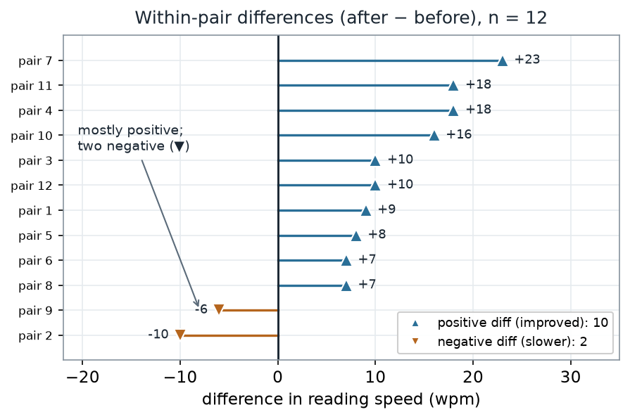
What to notice. Notice that the differences cluster tightly and mostly to the right of zero. That is the whole question in one picture: are these differences centered at zero (no typical change), or shifted positive? Two students slipped, so it is not unanimous — which is exactly why we need a test rather than a glance. We distinguish improvements from declines by marker shape (▲ vs ▼) and stem direction, not color alone.
The differences, as numbers (nonvisual equivalent).
| Summary | Value |
|---|---|
| n pairs | 12 |
| Positive differences (after > before) | 10 |
| Negative differences | 2 |
| Zero differences | 0 |
| Differences (wpm), sorted | −10, −6, +7, +7, +8, +9, +10, +10, +16, +18, +18, +23 |
| Median difference | +9.5 wpm |
Two questions, two tests
Both tests chase the same idea — no typical change — but under different assumptions. The sign test only needs the median within-pair difference to be zero (a subject is equally likely to get faster or slower); it makes no claim about the shape of the difference distribution. The signed-rank test asks more: it additionally assumes the differences are symmetric about zero, which is exactly what makes the \(\pm\) sign-flip enumeration on the ranked magnitudes valid. They also part company on how much of each difference they read. The sign test looks only at the sign (did this student get faster or slower?). The signed-rank test also uses the size of each change, through the rank of its absolute value. The shown R computes both — and there is no plotting in it; the picture is your PNG:
# matched pairs: reading speed before and after the program
before <- c(204, 226, 215, 180, 217, 219, 188, 196, 264, 176, 242, 176)
after  <- c(213, 216, 225, 198, 225, 226, 211, 203, 258, 192, 260, 186)
d <- after - before                        # the 12 within-pair differences

# sign test: is the number of positive differences surprising under Binomial(n, 1/2)?
n_pos <- sum(d > 0)
binom.test(n_pos, n = length(d), p = 0.5)  # exact two-sided sign test

# Wilcoxon signed-rank: rank |d|, sum the ranks that carry a + sign (W+).
# NOTE: |d| has ties here (7,7; 10,10,10; 18,18), so R cannot return an exact p — it warns
# ("cannot compute exact p-value with ties"), silently overrides exact = TRUE, and falls back to the
# tie-corrected normal approximation (p ~ 0.017). The exact 0.012 the notes report is the exact
# CONDITIONAL p from enumerating all 2^12 sign patterns on the tied ranks (see the signed-rank box below).
wilcox.test(after, before, paired = TRUE, exact = TRUE)
Worked example — the sign test
Throw away the magnitudes and keep only the signs: 10 of the 12 differences are positive. If the program did nothing — if getting faster or slower were a coin flip for each student — the count of positive differences would follow \(\text{Binomial}(12, \tfrac{1}{2})\), centered at 6. We observed 10.
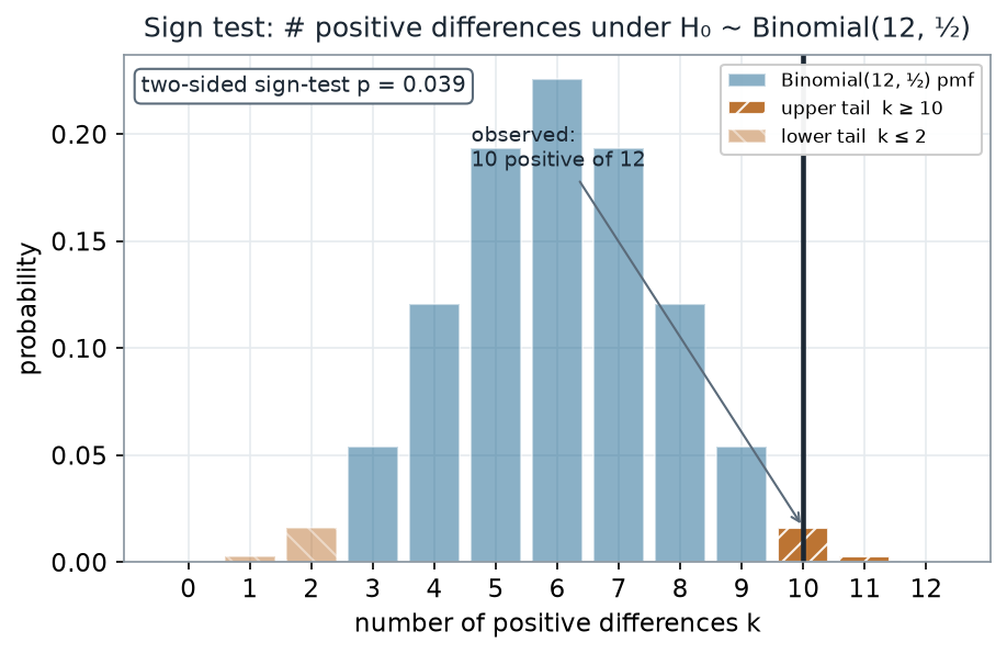
What to notice. The observed count of 10 is far from the center (6). The upper tail — outcomes at least as extreme as 10 positives — is \(P(X \ge 10) = \tfrac{66 + 12 + 1}{4096} = 0.0193\). By symmetry the two-sided \(p\)-value doubles it to about 0.039. We would reject “no typical change” at the 5% level. Note what the sign test never used: that some improvements were +23 while a slip was only −6. Every difference counted as a single tick mark.
Sign-test read-out (nonvisual equivalent).
| Quantity | Value |
|---|---|
| Positive differences observed | 10 of 12 |
| Null model | # positive \(\sim \text{Binomial}(12, \tfrac{1}{2})\) |
| Upper tail \(P(X \ge 10)\) | 0.0193 |
| Two-sided sign-test \(p\) | 0.039 |
Worked example — the Wilcoxon signed-rank test
The sign test is honest but blunt. The signed-rank test keeps more information: rank the absolute differences from smallest to largest, then add up the ranks that belong to positive differences. That sum is \(W^{+}\). Because two students slipped by only small amounts, their ranks are small, so they barely offset the many large positive ranks.
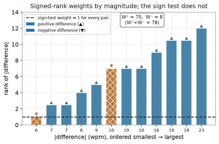
What to notice. Every bar’s height is the rank of that difference’s magnitude, so the +23 change (rank 12) counts twelve times as much as the smallest change (rank 1) — the sign test would have made them equal (the dashed line). The two negatives (▼, at \(|d| = 6\) and \(|d| = 10\)) sit low, so \(W^{-} = 1 + 7 = 8\) is tiny next to \(W^{+} = 70\). The two always sum to \(n(n+1)/2 = 78\). The exact two-sided \(p\)-value — from enumerating all \(2^{12}\) sign patterns on these ranks — is about 0.012, a bit smaller than the sign test’s, because the signed rank noticed that the improvements were large and the two declines were small.
Signed-rank read-out (nonvisual equivalent).
| Quantity | Value |
|---|---|
| Absolute differences, ranked (ties averaged) | 1, 2.5, 2.5, 4, 5, 7, 7, 7, 9, 10.5, 10.5, 12 |
| \(W^{+}\) (sum of positive-difference ranks) | 70 |
| \(W^{-}\) (sum of negative-difference ranks) | 8 |
| \(W^{+} + W^{-} = n(n+1)/2\) | 78 |
| Exact two-sided \(p\) | ≈ 0.012 |
Three of the absolute differences tie at 10 wpm and two tie at 7 and at 18; tied magnitudes share the average of the ranks they would occupy (three values at ranks 6–8 each become 7), which keeps the total fixed at 78.
Don’t unpair paired data
“Before and after are just two samples — run a two-sample test.” This throws away the pairing, and the pairing is the point. The spread across students here is about 27 wpm (some read 176, some 264); the average change is only about 9 wpm. An independent two-sample test drowns that 9-wpm signal in 27-wpm between-student noise. The paired difference, by contrast, cancels each student’s baseline, so the 12 changes have a spread of only about 10 wpm — the pairing shrinks the noise from about 27 wpm to about 10 wpm, removing well over half of the between-student spread. Unpairing is not a milder analysis; it is usually a weaker one, and it answers a different question.
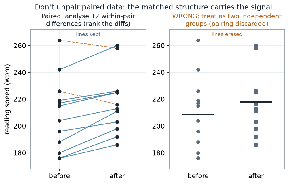
What to notice. On the left, individual lines mostly rise: student by student the change is clear. On the right, the two clouds overlap so much that the group means (208.6 → 217.8 wpm) look almost indistinguishable given the scatter. Same numbers, but the unpaired picture hides the signal the pairing reveals. Keep the lines.
Paired vs unpaired (nonvisual equivalent).
| Analysis | What it uses | Consequence |
|---|---|---|
| Paired (correct) | the 12 within-pair differences | cancels ~27 wpm between-student spread; 10 of 12 improve |
| Unpaired (wrong) | before-group vs after-group | keeps the large between-student spread; a ~9 wpm shift looks like noise |
Check your understanding (ungraded)
- In one sentence, why is the within-pair difference the right thing to analyze here, rather than the before and after readings separately?
- The sign test used only that 10 of 12 differences were positive. Reconstruct the two-sided \(p\)-value of 0.039 from \(\text{Binomial}(12, \tfrac{1}{2})\), and say in words what “at least as extreme” means.
- \(W^{+} = 70\) and \(W^{-} = 8\). Explain how you know these must sum to 78 before computing either one, and what a value of \(W^{+}\) near 39 would have told you.
- The signed-rank \(p\) (≈ 0.012) came out smaller than the sign-test \(p\) (≈ 0.039). Which feature of this data set made the signed rank more decisive — and describe a data set where the two tests would instead disagree in the other direction.
Reading guide
- OpenIntro Statistics 4e — inference for paired data — a conceptual companion to reducing pairs to differences; read for the intuition, then map it onto the difference lollipop above.
- IMS — inference for comparing paired means — reinforces “one difference per pair” as the unit of analysis, from the resampling side.
- Learning Statistics with R (Navarro) — the Wilcoxon signed-rank test — an instructor reference on the mechanics of ranking \(|d|\) and forming \(W^{+}\) (cited, not reproduced).
- NIST/SEMATECH e-Handbook — Wilcoxon signed rank test — a reference for the exact null and the large-sample approximation you will meet next.
Accessibility notes
Mathematics is live text (\(W^{+}\), \(\text{Binomial}(12, \tfrac{1}{2})\), and \(n(n+1)/2\) render as MathML, not images). Every figure carries an alt line stating its message, an adjacent “what to notice” reading, and a data-summary table, so each point survives without the picture. Improvements and declines are distinguished by marker shape (▲ vs ▼), stem direction, and hatching — never color alone — and the two rank tests are labeled directly on the bars. A clean lint and a clean render are evidence; the rendered assistive-technology review is a human step.
Assessment (descriptive only)
This week contributes learning evidence toward reducing paired data to differences and choosing and running a rank-based test of no-typical-change. That is the shape only; the actual graded prompts, points, and due dates live in Blackboard.
Public vs. graded. These are public, ungraded notes and practice. Graded prompts, keys, rubrics, point values, and due dates live in Blackboard Ultra, which governs.
Looking ahead
Next week we move from one paired sample to two independent groups and the Wilcoxon rank-sum (Mann–Whitney) test — where we pool both groups, rank everything together, and ask whether one group’s ranks pile up higher than the other’s. The ranking habit you built here carries straight over; only the null we resample against changes.