Week 2 — Order statistics, ranks & the ECDF
The assumption-light description toolkit every later method is built on
Source basis. Original instructor-authored notes; data is synthetic (30 “response times” in milliseconds drawn from a fixed generator, seed 45202, plus small demo sets). Open texts are conceptual companions cited by section title only (map-don’t-mine); no prose, figures, examples, or exercises are reproduced. See Open readings & attribution. Ungraded — Blackboard is authoritative for graded work.
This week. Last week we asked what is fragile here? and saw the mean and SD get dragged around by a single point. Before we resample or test anything, we need a description toolkit that does not lean on a distributional shape. Three objects give us exactly that — the empirical CDF, the order statistics, and the ranks. Every rank test, every quantile, and every distribution-free comparison in this course is built out of these three. Get them solid now and the rest of the semester is assembly.
Learning goals
By the end of this week you should be able to:
- Define and read the empirical CDF \(\hat F(x) = \#\{x_i \le x\}/n\), and use it to look up quantiles as inverse-ECDF lookups.
- Identify the order statistics \(x_{(1)} \le \dots \le x_{(n)}\) and locate the five-number summary at fixed positions in the sorted sample.
- Convert values to ranks, handling ties by averaging, and say why ranks are the raw material of the rank tests to come.
- Compare two groups with overlaid ECDFs and read stochastic ordering off the picture — no Normal assumption required.
- Explain what ranks keep (order) and what they discard (spacing).
Where we are
A histogram bins the data and throws away the exact values; a mean collapses everything to one number. The empirical CDF does neither. It is the sample’s own distribution function: at each value \(x\) it reports the proportion of observations at or below \(x\), \[\hat F(x) = \frac{\#\{x_i \le x\}}{n}.\] It is a step function that starts at 0, jumps by \(1/n\) at every observation, and ends at 1. Nothing is assumed about the population — \(\hat F\) is a complete, lossless summary of the sample, and every quantile we will ever read is read off it.
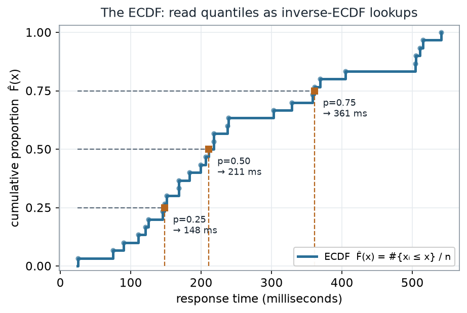
What to notice. A quantile is just an inverse-ECDF lookup. Because the curve is a step function, a height like 0.25 is reached at the first value whose cumulative proportion is at least 0.25 — here \(8/30 = 0.267\), so the 0.25-quantile is the 8th sorted value. There is no smoothing and no distribution to fit; the median (211 ms) is simply where the curve first reaches height 0.50.
The ECDF read-off (nonvisual equivalent).
| Height \(p\) | First cumulative proportion \(\ge p\) | Quantile (ms) |
|---|---|---|
| 0.25 | \(8/30 = 0.267\) | \(Q_1 = 148\) |
| 0.50 | \(15/30 = 0.500\) | median \(= 211\) |
| 0.75 | \(23/30 = 0.767\) | \(Q_3 = 361\) |
Order statistics: the sorted sample
Those look-ups landed on the 8th, 15th, and 23rd values in sorted order. Sorting the sample turns it into its order statistics \(x_{(1)} \le x_{(2)} \le \dots \le x_{(n)}\), where \(x_{(k)}\) is simply the \(k\)-th smallest value. Once sorted, the five-number summary lives at fixed positions and needs no formula beyond counting.
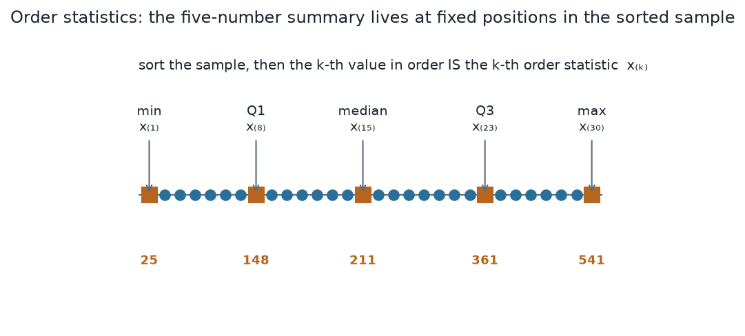
What to notice. The min, quartiles, median, and max are not special formulas — they are particular order statistics. The whole apparatus of “position in the sorted list” is what makes these summaries distribution-free: reorder the world however you like, \(x_{(15)}\) is still the 15th smallest value.
Five-number summary as order statistics (nonvisual equivalent).
| Summary | Order statistic | Value (ms) |
|---|---|---|
| Minimum | \(x_{(1)}\) | 25 |
| \(Q_1\) | \(x_{(8)}\) | 148 |
| Median | \(x_{(15)}\) | 211 |
| \(Q_3\) | \(x_{(23)}\) | 361 |
| Maximum | \(x_{(30)}\) | 541 |
Worked example — reading quantiles off the ECDF
The R you would run is short, and notice there is no plotting in it — the picture above is downstream:
# Schematic: the named data objects are the sample(s) described in the text above; this illustrates the analysis, not a self-contained runnable block.
# read quantiles as inverse-ECDF lookups; no plotting here
x    <- response_times                       # the 30 observed values (ms)
Fhat <- ecdf(x)                              # the empirical CDF, a step function
sort(x)[c(8, 15, 23)]                        # Q1, median, Q3 as order statistics x_(8), x_(15), x_(23)
quantile(x, c(.25, .5, .75), type = 1)       # the SAME values, as inverse-ECDF (type-1) quantiles
Both lines return 148, 211, 361. The second line names the convention explicitly: type = 1 is the inverse of the ECDF — the smallest value whose cumulative proportion reaches \(p\). Other software defaults (R’s type = 7, for instance) interpolate between order statistics and can give slightly different numbers; when you compare tools, state which quantile definition you used.
Ranks: replace each value by its position
Ranks push the order-statistic idea one step further: instead of keeping the values, keep only where each value falls in the sorted order. The smallest gets rank 1, the next rank 2, and so on. The one wrinkle is ties: when several observations are equal, they cannot each claim a different position, so each gets the average of the positions they jointly occupy.
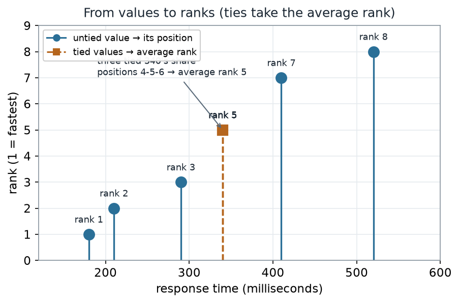
What to notice. Ties are resolved by averaging, not by breaking ties arbitrarily: \((4+5+6)/3 = 5\). This keeps the sum of ranks fixed at \(1+2+\dots+n\) no matter how many ties occur, which is exactly the property the rank tests in Weeks 7–8 rely on.
Values to ranks, with a tie (nonvisual equivalent).
| Sorted value (ms) | 180 | 210 | 290 | 340 | 340 | 340 | 410 | 520 |
|---|---|---|---|---|---|---|---|---|
| Position | 1 | 2 | 3 | 4 | 5 | 6 | 7 | 8 |
| Rank (average ties) | 1 | 2 | 3 | 5 | 5 | 5 | 7 | 8 |
Worked example — from values to ranks
# Schematic: the named data objects are the sample(s) described in the text above; this illustrates the analysis, not a self-contained runnable block.
# ranks with the default average-ties rule; no plotting here
demo <- c(210, 340, 340, 180, 520, 410, 290, 340)
rank(demo)                                   # ties.method = "average" is R's default
#  -> 2 5 5 1 8 7 3 5   (the three 340's each become (4+5+6)/3 = 5)
rank() returns the ranks in the original order of the data, so the three 340’s — the 2nd, 3rd, and 8th entries of demo — all come back as 5. Everything downstream (rank sums, signed ranks) is arithmetic on this vector.
Comparing two groups without a model
Because the ECDF assumes nothing about shape, we can lay two groups’ ECDFs on the same axes and compare them distribution-free. If one curve sits entirely to the right of the other, that group tends to produce larger values — it is stochastically larger.
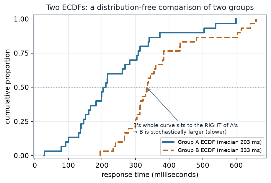
What to notice. We did not assume Normality, equal variance, or even a specific shape. “B is to the right of A” is a statement about whole distributions. It is this right-shift — the whole B curve sitting to the right, equivalently the area between the two ECDFs (how often a Group B value lands above a Group A value) — that seeds the two-sample rank-sum / Mann-Whitney methods in Week 8. A different summary, the largest vertical gap between the two curves (here about 0.57), is the two-sample Kolmogorov-Smirnov statistic — a distinct EDF-based test we do not meet in Week 8, so keep the two apart.
Two-group comparison (nonvisual equivalent).
| Group | Median (ms) | Position relative to the other |
|---|---|---|
| A | 203 | ECDF to the left (smaller values) |
| B | 333 | ECDF entirely to the right (stochastically larger) |
| Both | — | max vertical ECDF gap \(\approx 0.57\) (two-sample Kolmogorov-Smirnov statistic, not the Week 8 rank test) |
A common mistake
“Ranks capture the data, so I can throw the raw values away.” Ranks capture the order and nothing else. Two datasets can have the identical rank vector while their raw values are spaced completely differently — one tightly clustered, the other stretched across a huge range. Any conclusion that depends on how far apart the values are (a mean difference, an effect size in real units) is invisible to ranks. Rank methods trade that information away on purpose in exchange for robustness; that trade is a choice, not a free lunch.
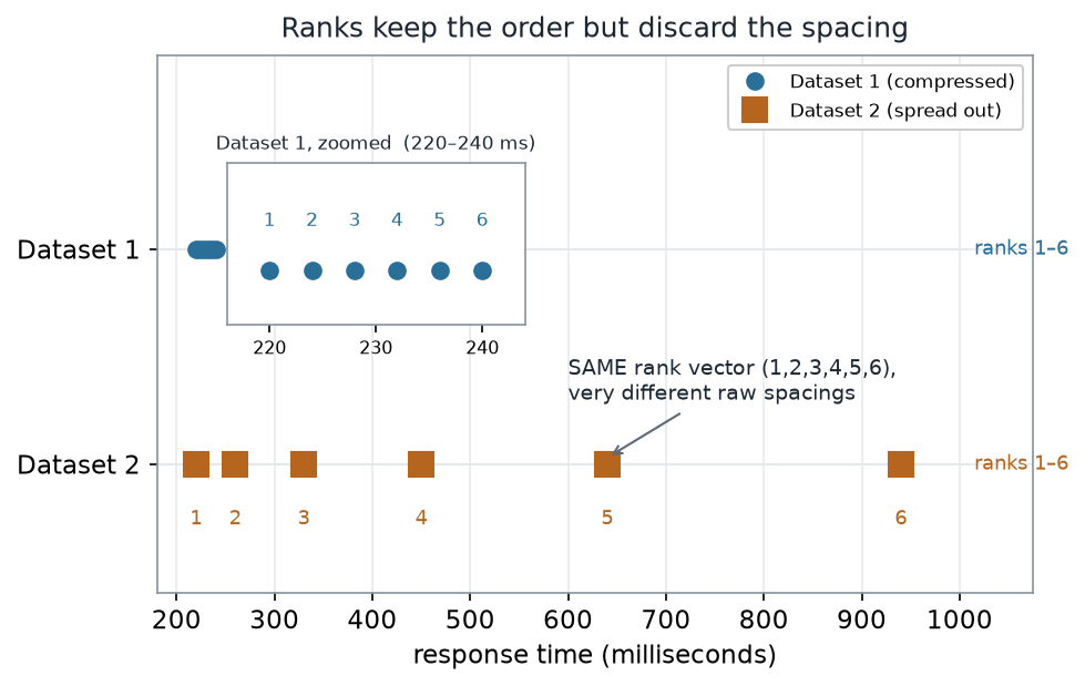
What to notice. Both rows produce exactly \((1,2,3,4,5,6)\), so any rank-based summary treats them as identical — yet Dataset 2’s range is 36× wider than Dataset 1’s. Ranks answer “which is bigger?”, never “by how much?”
Same ranks, different spacing (nonvisual equivalent).
| Dataset | Values (ms) | Rank vector | Range (ms) |
|---|---|---|---|
| 1 (compressed) | 220, 224, 228, 232, 236, 240 | 1, 2, 3, 4, 5, 6 | 20 |
| 2 (spread out) | 220, 260, 330, 450, 640, 940 | 1, 2, 3, 4, 5, 6 | 720 |
Check your understanding (ungraded)
- Explain in one sentence why \(\hat F(x)\) is a step function and why every jump has the same height.
- Using the inverse-ECDF rule, which order statistic is the 0.90-quantile of a sample of \(n=30\)? (Give the subscript \(x_{(k)}\).)
- A sample has four observations equal to 12, and they occupy positions 5, 6, 7, 8 in sorted order. What average rank does each receive, and why does averaging keep the total rank sum unchanged?
- Two ECDFs cross each other (neither is entirely to the right). Can you still say one group is stochastically larger? What would you report instead?
- Give one real question the ranks of a dataset can answer and one they cannot.
Reading guide
- OpenIntro Statistics 4e — Examining numerical data — a companion for quantiles and the five-number summary; read for intuition, then check it against the ECDF picture above.
- IMS — Exploring numerical data — reinforces distributions and quantiles as descriptive objects.
- NIST/SEMATECH e-Handbook — Empirical Distribution Function; Percentiles — a reference for the ECDF definition and for how percentile conventions differ (the
typeissue). - Learning Statistics with R (Navarro) — Descriptive statistics — an R-oriented reference for percentiles and
rank()(cited, not reproduced).
Accessibility notes
Mathematics is live text (\(\hat F(x) = \#\{x_i \le x\}/n\) renders as MathML, not an image). Every figure carries an alt line stating its message, a “what to notice” reading, and an adjacent data-summary table, so each point survives without the picture. Series are distinguished by linestyle and marker (solid circle = observed/untied, dashed square = second group/tied) plus value-bearing labels, never color alone. A clean lint and a clean render are evidence; the rendered assistive-technology review is a human step.
Assessment (descriptive only)
This week contributes learning evidence toward reading an ECDF and its quantiles, working with order statistics and ranks, and making a distribution-free two-group comparison. That is the shape only; the actual graded prompts, points, and due dates live in Blackboard.
Public vs. graded. These are public, ungraded notes and practice. Graded prompts, keys, rubrics, point values, and due dates live in Blackboard Ultra, which governs.
Looking ahead
Next week we put these objects to work. The ranks and order statistics you built here become the currency of resampling-based tests: we hold the pooled values fixed, shuffle the group labels, and let the ECDF-style comparison you just met turn into a permutation p-value.