Lab 5 — A small simulation study
Measuring Type I error and power for two tests under conditions you control
Source basis. Original instructor-authored lab; all data is synthetic, generated by a fixed simulation (seed 45225) — no real dataset is used. Open texts are conceptual companions cited by section title only (map-don’t-mine); no prose, figures, examples, or exercises are reproduced. See Open readings & attribution. Public and ungraded — Blackboard is authoritative for graded lab prompts, points, and due dates. Pairs with Week 13.
This lab. Every earlier lab handed you one dataset and asked what a method says about it. Here we flip the telescope around: we invent the truth, generate data from it thousands of times, and watch how often each test gets the answer right. That is a simulation study — the way statisticians actually decide when to reach for the t-test and when to reach for a rank test.
Learning goals
By the end of this lab you should be able to:
- Write a simulation loop: fix a truth, generate data, apply competing methods, record the outcome, and repeat.
- Estimate a test’s Type I error (rejection rate when the null is true) and its power (rejection rate when the null is false), and read them off a picture.
- Explain why a rank test can out-power the t-test under heavy tails — and confirm both tests still control Type I error.
- Attach a Monte Carlo standard error to any simulated rate, and say how many replications you need.
The simulation loop
A simulation study is a single idea run in a loop. You choose a truth — a data-generating process (DGP) and, if you want power, a real effect. You generate data from that truth, apply every method you are comparing, and record what each one decided. Then you do it again, thousands of times, and summarize how often each method landed where you wanted. Because you set the truth, you know the right answer, so you can grade the methods.
Our study compares two two-sample tests on groups of n = 20 each, both two-sided at α = 0.05: the Welch t-test and the Wilcoxon rank-sum (Mann–Whitney) test. Two data-generating processes stand in for “well-behaved” and “misbehaved” data: a Normal DGP and a heavy-tailed one (a Student t with 3 degrees of freedom, rescaled to unit variance so a shift is measured in standard deviations).
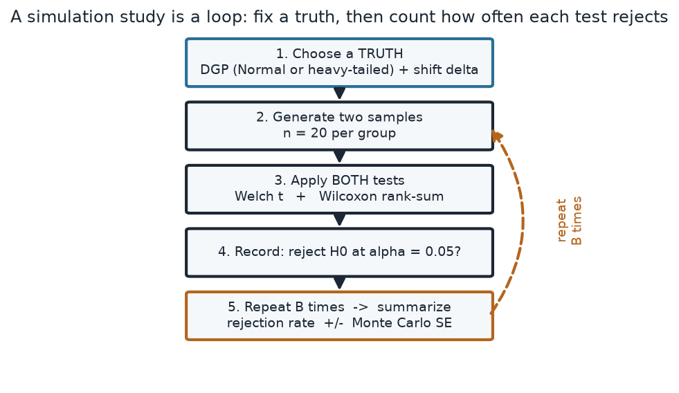
What to notice. Nothing here is about our particular data — it is about the procedure. The loop touches real data zero times; it manufactures data from a truth we chose. The thing we estimate is not a mean or a median but a property of a test: how often it rejects. Change the truth in step 1 and the same loop measures Type I error (no real effect) or power (a real effect).
The loop, as steps (nonvisual equivalent).
| Step | What happens |
|---|---|
| 1 | Choose a truth: a DGP (Normal or heavy-tailed) and a shift δ |
| 2 | Generate two samples, n = 20 each |
| 3 | Apply both tests: Welch t and Wilcoxon rank-sum |
| 4 | Record whether each rejects H₀ at α = 0.05 |
| 5 | Repeat B times; summarize as a rejection rate ± Monte Carlo SE |
The R is a loop, and — as always in these labs — it contains no plotting; the pictures below are the downstream summary:
# one simulation study: fix a truth, then count how often each test rejects
set.seed(45225)
rheavy <- function(n) rt(n, df = 3) / sqrt(3)   # t_3 standardized to unit variance

sim_once <- function(n, shift, rdata) {
  a <- rdata(n)                                  # group A (the null group)
  b <- rdata(n) + shift                          # group B, shifted by `shift`
  c(t      = t.test(a, b)$p.value      < 0.05,   # Welch t-test rejects?
    wilcox = wilcox.test(a, b)$p.value < 0.05)   # Wilcoxon rank-sum rejects?
}

B      <- 5000
result <- replicate(B, sim_once(n = 20, shift = 0, rdata = rheavy))
rowMeans(result)                                 # a rejection rate for each test
Worked example — Type I error under two nulls
Set the shift to δ = 0 (the two groups share one distribution, so the null is true) and run the loop B = 5000 times under each DGP. A well-behaved test should reject about 5% of the time — no more, or it is crying wolf.
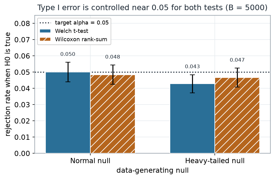
What to notice. Both tests control Type I error near 0.05 under both DGPs — the small departures (the t-test’s 0.043 under heavy tails, for instance) are inside Monte Carlo noise, not a real defect. This is the price of admission: a test that rejected far more than 5% under the null would be disqualified before we ever discussed power. Because both tests pass, the power comparison that follows is a fair fight.
Type I error read-out (nonvisual equivalent).
| Data-generating null | Welch t-test | Wilcoxon rank-sum |
|---|---|---|
| Normal | 0.050 (±0.003) | 0.048 (±0.003) |
| Heavy-tailed (\(t_3\)) | 0.043 (±0.003) | 0.047 (±0.003) |
(B = 5000; the ± is one Monte Carlo standard error.)
Worked example — power under heavy tails
Now give the two groups a genuine difference. Keep the heavy-tailed DGP and shift group B by a location amount δ, measured in standard deviations, from 0 up to 2.5. At each δ we rerun the loop and record how often each test rejects — that rejection rate is the power.
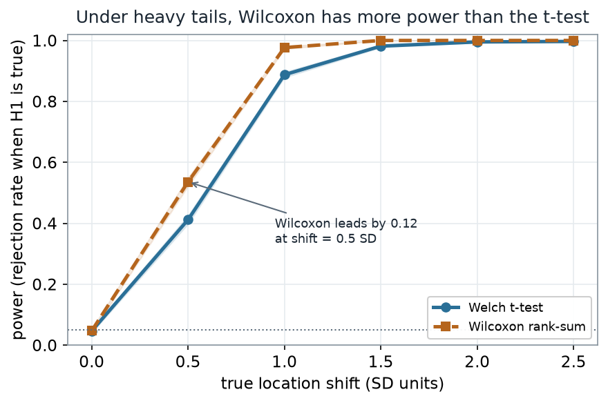
What to notice. Both curves rise from ≈ 0.05 (the Type I error, when δ = 0) toward 1. But the dashed Wilcoxon curve is above the solid t-curve through the whole climb: at a half-SD shift it catches a real difference 54% of the time versus the t-test’s 41%. Heavy tails throw occasional wild values that inflate the t-test’s standard error and blunt it; the rank test only cares about order, so those wild values cannot drag it around. Where the shape is heavy-tailed, the rank test is the more powerful choice.
Power read-out under heavy tails (nonvisual equivalent).
| Shift δ (SD) | Welch t power | Wilcoxon power |
|---|---|---|
| 0.0 | 0.047 | 0.047 |
| 0.5 | 0.412 | 0.536 |
| 1.0 | 0.888 | 0.977 |
| 1.5 | 0.981 | 1.000 |
| 2.0 | 0.995 | 1.000 |
| 2.5 | 0.997 | 1.000 |
(B = 5000 per shift. The two tests tie only at δ = 0, where “power” is just the Type I error.)
A common mistake
“I ran the simulation and Wilcoxon’s power was 0.51, so that’s the answer.” A single simulation run is itself a random experiment. Its estimate has a Monte Carlo standard error, and with too few replications that error is large enough to flip your conclusion. The number you print is not the truth — it is one draw from a distribution centered on the truth. Report it with its Monte Carlo SE, and make B big enough that the SE is small relative to the difference you care about.
How many replications? Monte Carlo error
For a rejection rate \(\hat p\) estimated from \(B\) independent runs, the Monte Carlo standard error is \(\sqrt{\hat p(1-\hat p)/B}\) — the ordinary standard error of a proportion. It shrinks like \(1/\sqrt{B}\), so cutting the error in half costs four times the runs. To see it, we fix one configuration (heavy tails, δ = 0.5 SD, the Wilcoxon test) and watch a single study’s estimate evolve as its replications accumulate.
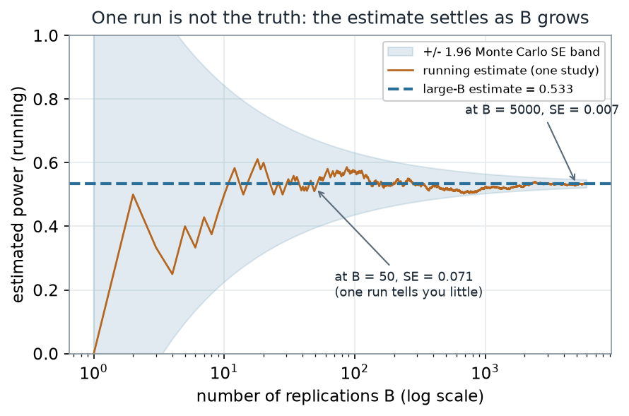
What to notice. Early on, the running estimate lurches between 0.25 and 0.6 — at B = 50 the SE is 0.071, so a lone small run could report anything from 0.4 to 0.7 and none of it would mean much. As B grows the band closes in and the line pins down near 0.533; at B = 5000 the SE is 0.007. The lesson is not “use 5000” as a rule — it is that the number you need depends on how small an error you can tolerate, and you can compute it in advance from \(\sqrt{\hat p(1-\hat p)/B}\).
Monte Carlo SE vs. replications (nonvisual equivalent).
| Replications B | Monte Carlo SE of the rate |
|---|---|
| 50 | 0.071 |
| 100 | 0.050 |
| 500 | 0.022 |
| 1000 | 0.016 |
| 5000 | 0.007 |
(Configuration: heavy tails, δ = 0.5 SD, Wilcoxon; large-B estimate ≈ 0.533.)
The SE is a two-line calculation you can run before committing to a B:
# Monte Carlo standard error of an estimated rejection rate
p_hat <- 0.533
B     <- 5000
mc_se <- sqrt(p_hat * (1 - p_hat) / B)   # ~ 0.007; to halve it, quadruple B
Check your understanding (ungraded)
- In your own words, what does a simulation study estimate — and why does knowing the truth in step 1 make that estimate possible?
- Under the heavy-tailed null the t-test rejected 0.043 of the time and Wilcoxon 0.047. Are these evidence that one test is “better” at controlling Type I error? Use the Monte Carlo SE to decide.
- Both power curves pass through ≈ 0.05 at δ = 0. Explain why that single point is really the Type I error in disguise.
- You want a power estimate accurate to a Monte Carlo SE of about 0.01. Roughly how many replications does \(\sqrt{\hat p(1-\hat p)/B}\) tell you to run near \(\hat p = 0.5\)? Near \(\hat p = 0.05\)?
Reading guide
- IMS — Decision errors (Type I and Type II) — a conceptual companion for what the two error rates mean; read it, then match the definitions to the two bar heights above.
- OpenIntro Statistics 4e — Inference and the significance level — reinforces α as the target Type I rate the simulation is checking.
- Learning Statistics with R (Navarro) — Comparing two means / errors in hypothesis testing — a companion on the t-test vs. rank-test choice this lab measures empirically.
- NIST/SEMATECH e-Handbook — Assessing the power of a test by simulation — an instructor reference on estimating power computationally (cited, not reproduced).
Accessibility notes
Mathematics is live text (\(\sqrt{\hat p(1-\hat p)/B}\) renders as MathML, not an image). Every figure carries an alt line stating its message, a “what to notice” reading, and an adjacent data-summary table, so each point survives without the picture. The two tests are distinguished by linestyle and marker and hatch (t-test = solid line / round marker / solid bar; Wilcoxon = dashed line / square marker / hatched bar) and by labels, never by color alone. A clean lint and a clean render are evidence; the rendered assistive-technology review is a human step.
Assessment (descriptive only)
This lab contributes learning evidence toward building a simulation loop and estimating and interpreting Type I error, power, and Monte Carlo error. That is the shape only; the actual graded prompts, point values, and due dates live in Blackboard.
Public vs. graded. This is a public, ungraded lab exemplar. Graded lab prompts, keys, rubrics, point values, and due dates live in Blackboard Ultra, which governs.
Looking ahead
You now have the tool that settles method arguments empirically: don’t guess whether the t-test or a rank test wins on your kind of data — simulate it. In the project you will use exactly this loop as a sensitivity check, asking not only “what does my method say?” but “how often would a method like this get it right on data like mine?”